Intermediate Functions

In this lesson we will work with some more functions.

LEFT() and RIGHT() are some useful functions for separating out a part text that exists inside of a larger string of text.

We can also use CONCAT() to join multiple cells into one string of text.

If we want to check for multiple things to select a part of our data we might need functions like AND() and OR().

What can we do if we want to count or add up just a portion of our data that meets a certain criteria? The COUNTIF() and SUMIF() functions can help us out!

Download File

• Click to download the file.
• From the main office.com screen, upload the file from your download folder.

LEFT(), RIGHT() and CONCAT() worksheet

Both the LEFT() and RIGHT() functions extract the number of characters that you ask for from a cell reference. Their names indicate from which end of the text they start.

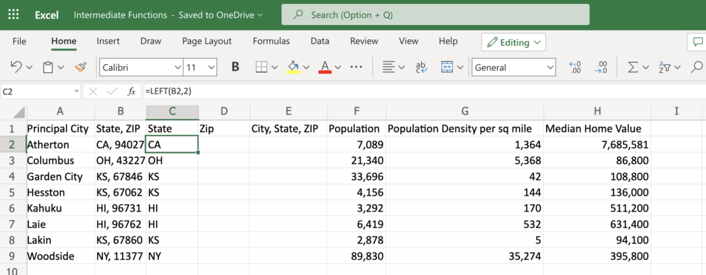
Try extracting the state abbreviation from B2.

• Start entering the formula in C2 because that is where you want the information to end up.
• Use LEFT() to start extracting from the left side. So start with =LEFT(
• Then enter the cell from which you want to extract the characters. =LEFT(B2,
• Now tell the function how many characters you want. =LEFT(B2,2)
• Great! Now copy the formula down to the bottom of the data.

This is how it should look.

Now extract the ZIP code from B2 into D2.

• You will need to use the RIGHT() function
• Don’t forget to ask for 5 characters. Note that this function works from the right and counts to the left.
• Copy the formula down to the bottom of the data.

Not only is it easy to separate information out, it is also easy to join information together!

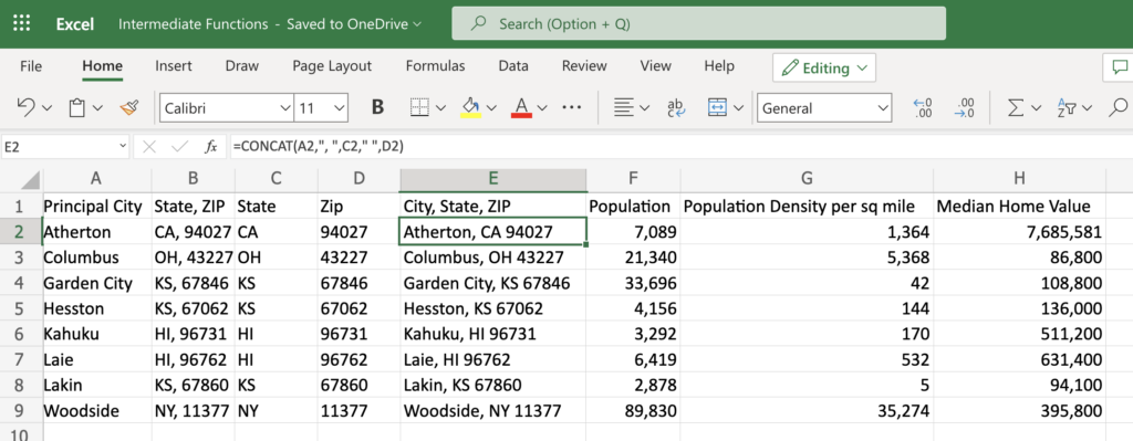
Let’s joint or concatenate the City together with the State and ZIP.

• Start by entering your formula in row 2 of column E (City, State, ZIP)
• You need to give the CONCAT() function all the items you want it to put together. Separate each one with a comma. Like this: =CONCAT(A2,C2,D2)
• What’s wrong? Is everything all ran together? That is because we have to explicitly tell the CONCAT() function where we want commas and spaces.
• Try adding a comma and space between the City and State. You will need to put any text that doesn’t come from a cell reference inside quotes. Like this: =CONCAT(A2,”, “,C2,D2). That is how the CONCAT() function can tell the difference between when you are using a comma to separate values and when you want it to include the comma in the joined text.
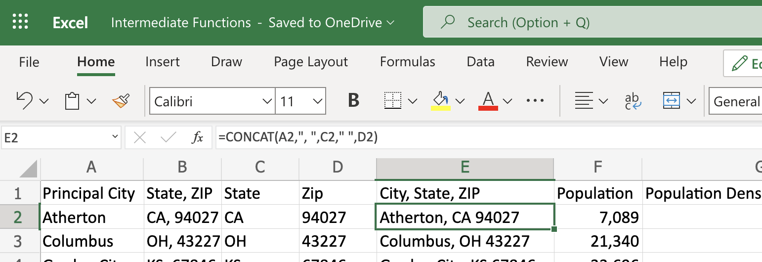
• Now add just a space between the State and ZIP!

Here is what the worksheet should look like now.

AND() and OR() Worksheet

Sometimes you will need to identify data by multiple criteria. Maybe two or three things need to be true about the data before it meets your criteria. It could also be that if any of serveral things are true it would meet your criteria. This is exactly what the AND() and OR() functions are for!

To use either function you give them a list of logical test separated by commas.

The AND() function finds FEWER results the more criteria or logical test you give it. This is because the all have to be true. Hence the name. Criteria one needs to be met AND criteria two and so forth.

The OR() function is very different. It finds MORE results the more criteria you give it. Once again the name explains how it works. If logical test one OR logical test two is true then it accepts it as correct.

Both of these functions display their findings as true or false.

Let’s get started.

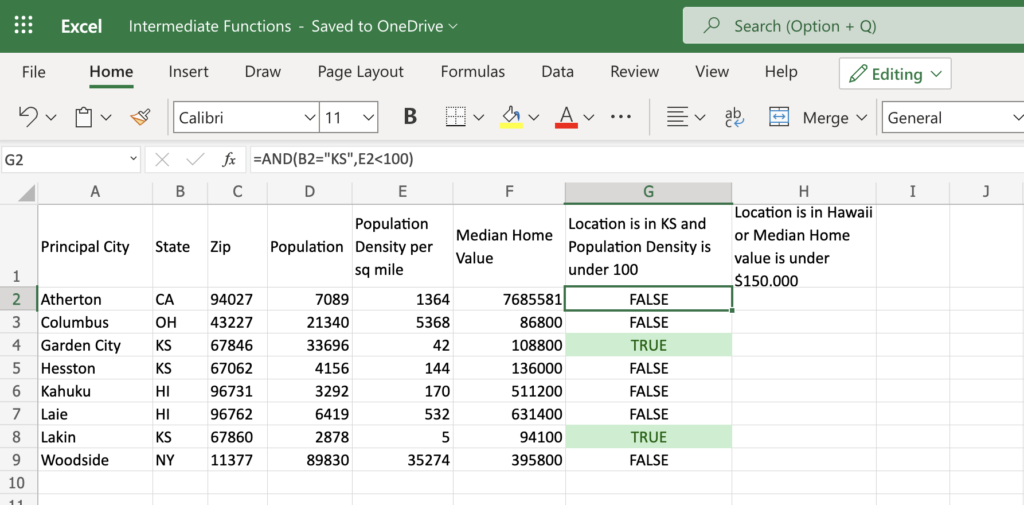
• In G2 build a formula with that checks if the State=KS and that the population density<100.
• The logical tests are separated by a comma so it will be: =AND(B2=”KS”, ??) Where the question marks are you will need to enter the second logical test.
• Copy the formula down to the bottom of the data.
• Do you remember how to highlight cell with conditional formatting? Review that lesson if needed. Then hight light all the cell that say “TRUE” with green.

The result should look like this.

Now let’s find rows where either of two test are true. Maybe we are looking for a place to live where the houses usually don’t cost over $150,000 but we would really like to live in Hawaii so we want to see those rows as well. Even if the normal cost of housing is higher than $150,00. In this example we want to find the rows where either the location is in Hawaii OR the median home value is under $150.000.

Are you ready to start?

• Enter your formula in H2.
• You will need to use the OR() function.
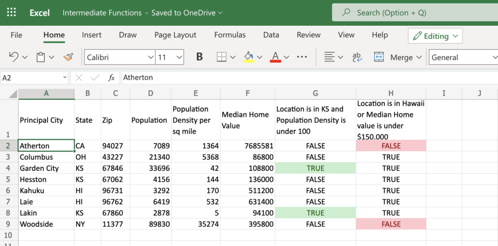
• Remember you are finding rows where the State=’HI’ OR the Median Home Value<150000.
• OK, write the formula. It’s very similar to the one you just did using the AND() function.
• Let’s do some conditional formatting again. This time highlight all the cell that say “FALSE” with red.

Does your worksheet look like the one below? If not, see if you can fix it.

COUNTIF() and SUMIF() Worksheet

It’s often very useful to count or total only items or rows that meet certain criteria. The COUNTIF() and SUMIF() functions are perfect for this.

They work just like their non-if versions except you can give them a logical test. Just enter the range as usual then a comma and then the logical test.

Let’s start with COUNTIF(). We’ll find the number of locations in Kansas. This time we’ll use the

• Enter your formula in B13
• Enter the range: =COUNTIF(B2:B9
• Now finish with the logical test. It needs to be in quotes. =COUNTIF(B2:B9,”=KS”)

You can also do it with your mouse with less typing if you prefer. Watch the video to see how.

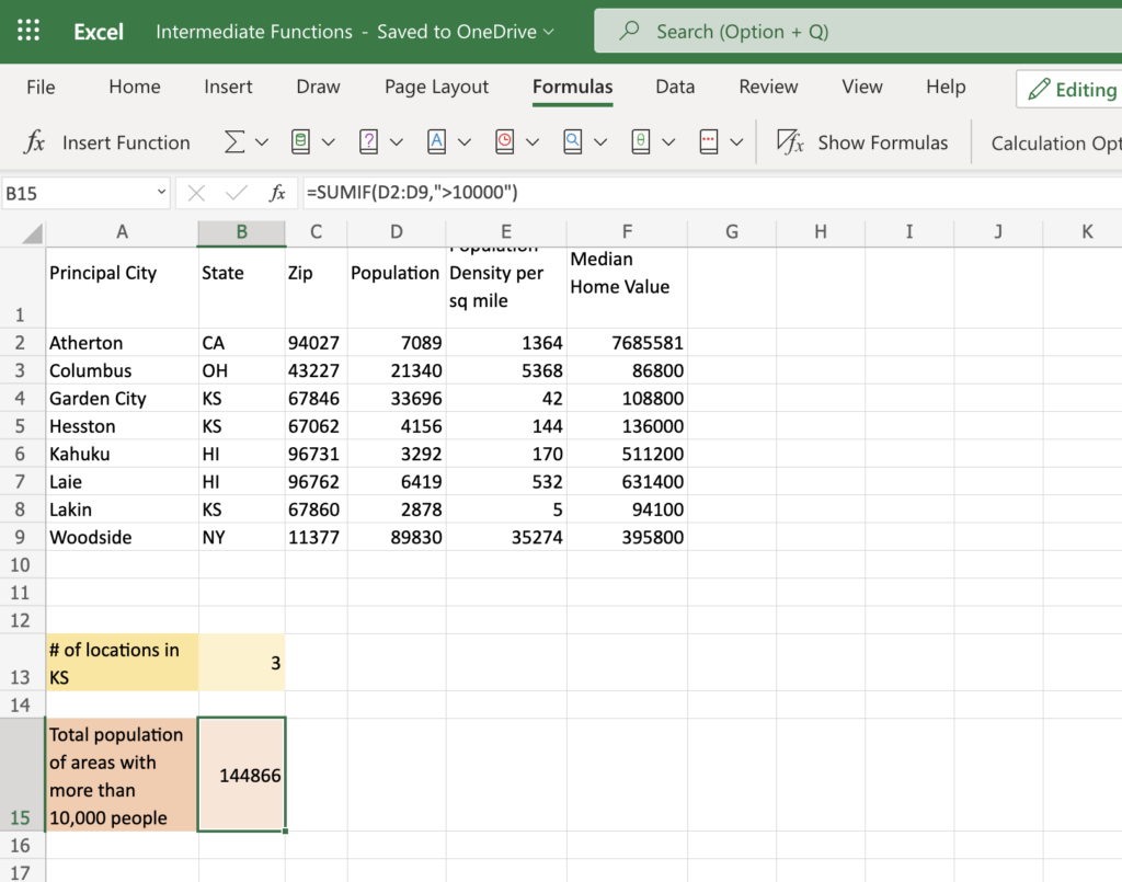
Now find the total population of areas with more the 10,000 people.

• Use the SUMIF() function in B15
• Is very much like the COUNTIF() example except the range will be D2:D9 and Population>10000.

The worksheet should look like this when you finish.

Great job!