VLOOKUP() Function

VLOOKUP stands for “Vertical Lookup”. It is a function that makes Excel search for a certain value in a column, the “table array”, in order to return a value from a different column in the same row.

Download File

• Click to download the file.
• From the main office.com screen, upload the file from your download folder.

VLOOKUP() False Worksheet

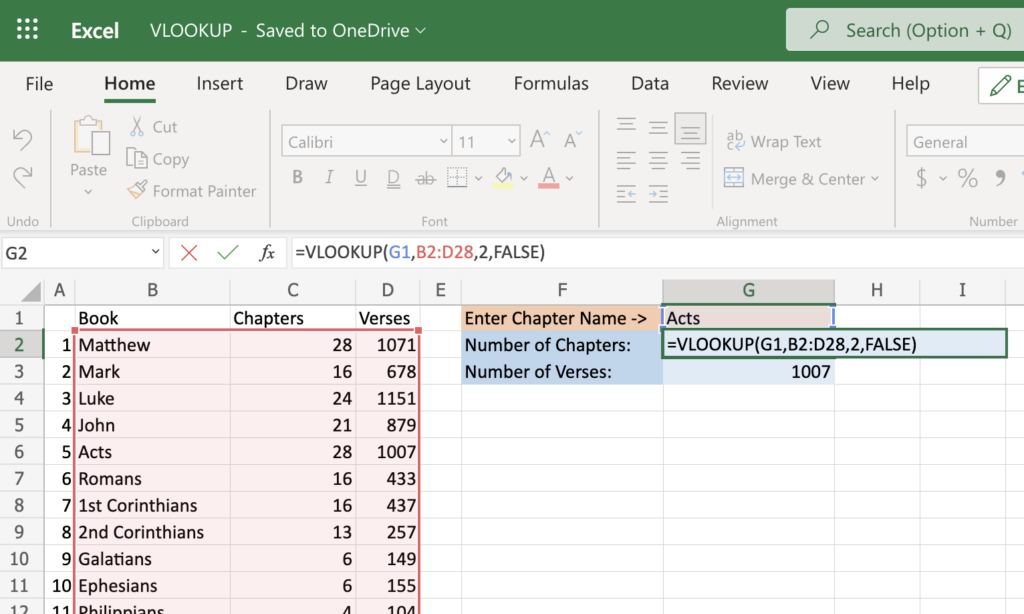
Start by entering a VLOOKUP() function in G2.

The VLOOKUP() function has 4 components. Use the Following screen shot for reference.

• #1 – First is the value you want to look up. In this example we are giving VLOOKUP() the book name from G1.
• #2 – The range in which you want to find the value and the return value. This is B2:D28. VLOOKUP() always searches in the leftmost column of the range. In our example this is column B or the column containing the book names. Note: The column you want to search needs to be to the left of the column that has the information you want to return. If it isn’t, you will need to rearrange the columns so that it is. In our case it is already on the left so we don’t need to move any columns.
• #3 – The number of the column within your defined range that contains the return value. In our case is the “Chapters” column or column C. We have to tell VLOOKUP to get the answer from column 2. This is because it is the 2nd column in the range we gave VLOOKUP() in the last step.
• #4 – We will enter “FALSE” 0 or FALSE tells VLOOKUP() that we want an exact match with the value you are looking for. 1 or TRUE tells VLOOKUP() to look for an approximate match. When working with text you will almost always use FALSE for exact match.

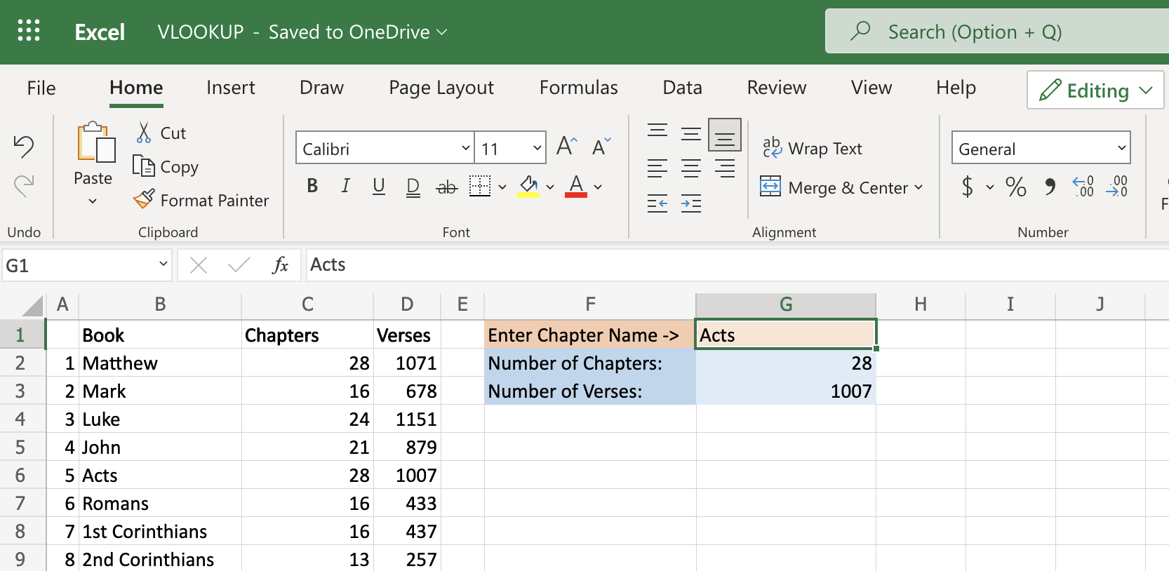
OK! Now you should be able to enter a book of the New Testament in G1 and get the number of chapters back in G2.

• Now write a formula in G3 that will display the number of verses. It will be very similar to the formula you just wrote. But the column number will be different.
• Enter different books into the G1 cell and watch the “Number of Chapters” and “Number of Verses” change!
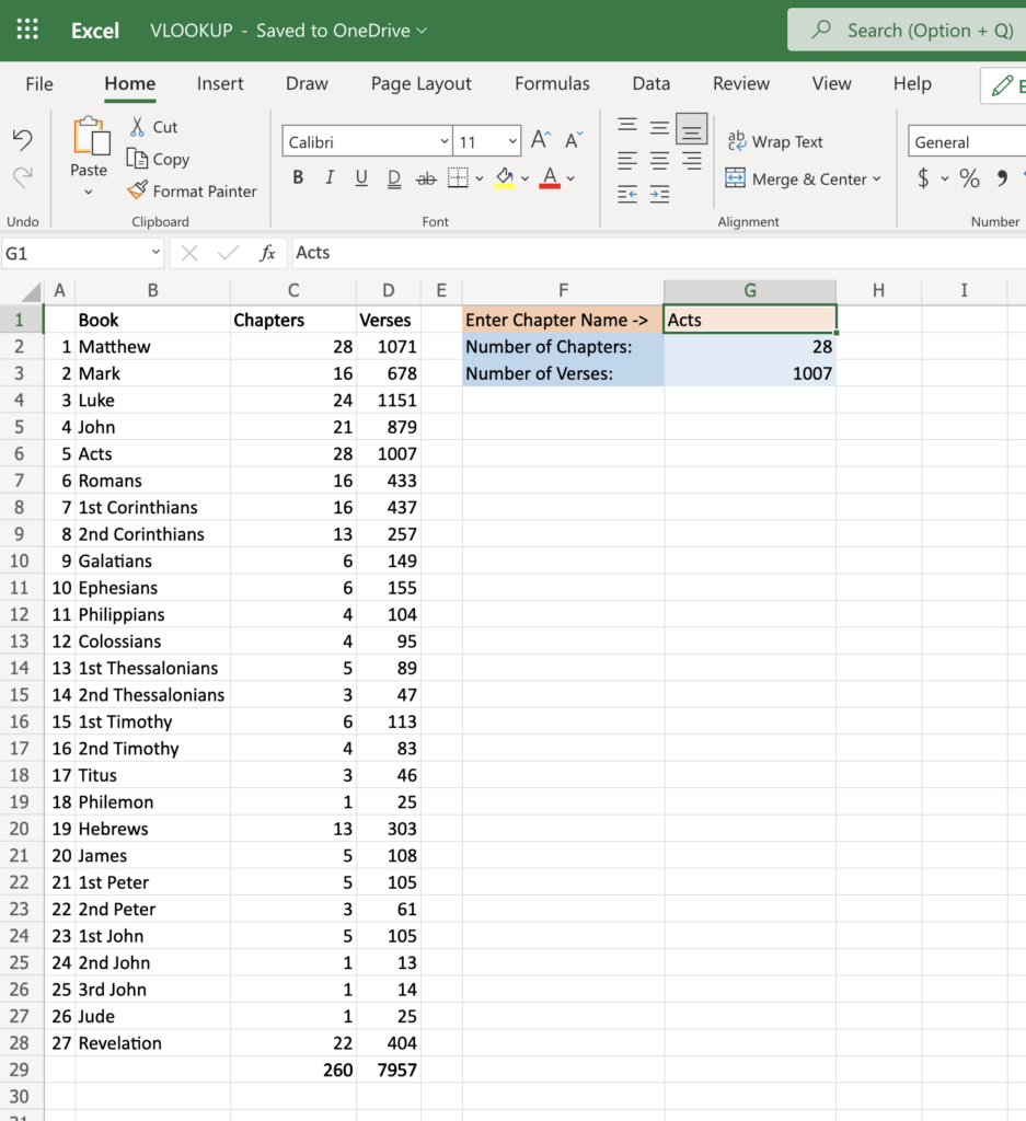
• To make your information even more interesting, add totals using the SUM() function at the bottom of columns C and D. This will tell us how many chapters and verses are in the New Testament.
• Another thing you can do to make the data look better is make the top row bold. Simply select the cell across the top of the table of data and then click the bold button on the “Home” menu.
• Go ahead and make the totals bold as well.

Here is a screenshot of the completed worksheet.

VLOOKUP() True Worksheet

It is possible to use VLOOKUP() to find a close match. That is what the “True” setting is for. This is most useful when searching for numbers.

The data needs to be in the correct order for this to work correctly. Just like before, the column you want to search for a match need to be the leftmost of the range.

Additionally the data in the column you are searching need to be sorted ascending. This is because VLOOKUP() goes down the column looking for a match. If it doesn’t find an exact match, it goes until it finds a value that is larger the the one it is looking for. It then stops and returned the previous value. In other words it returns the value that is closed to what you are searching for but is smaller. There could possibly be a value that is even closer to the target. But if it is larger than the searched for value it will not be returned. The returned answer will always be exactly the same or smaller than the search value.

You don’t need to worry about sorting this data though. It is already sorted correctly.

OK, let’s give it a try!

• Start by typing your formula into cell F2
• Enter: “=VLOOKUP(F1” This tells VLOOKUP() to search for data that match what is in cell F1
• Type a comma and continue with the range: =VLOOKUP(F1,A2:C28
• Now another comma and enter the row number that has the answer you want to return.
• One more comma and then enter True and then the closing parenthesis.

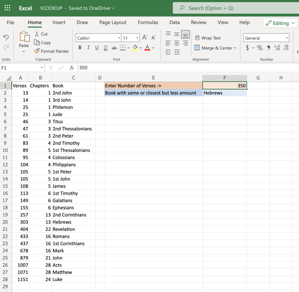
Does your worksheet look like this?

Experiment with entering different numbers in cell F1.

If you enter a number that is exactly what a book has it should return the name of that book.

If you enter a number that is not in the list it should find the closest one that is smaller.