Conditional Formatting

Conditional formatting is a wonderful way to draw attention to specific data. It also if very effective at highlighting differences in cell values. You will find other great uses for conditional formatting as you continue to use Excel.

Download File

• Click to download the file.
• From the main office.com screen, upload the file from your download folder.

Data Bars Worksheet

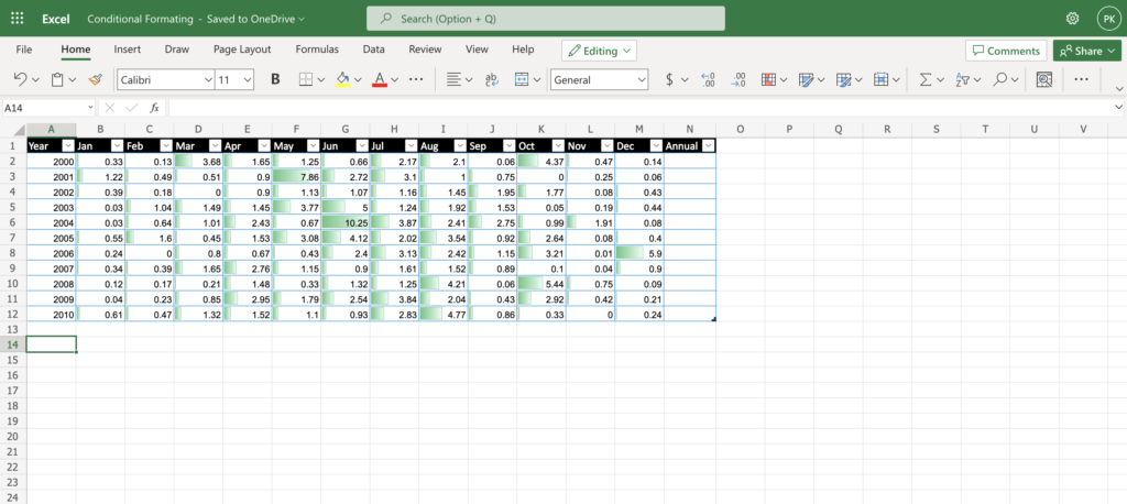
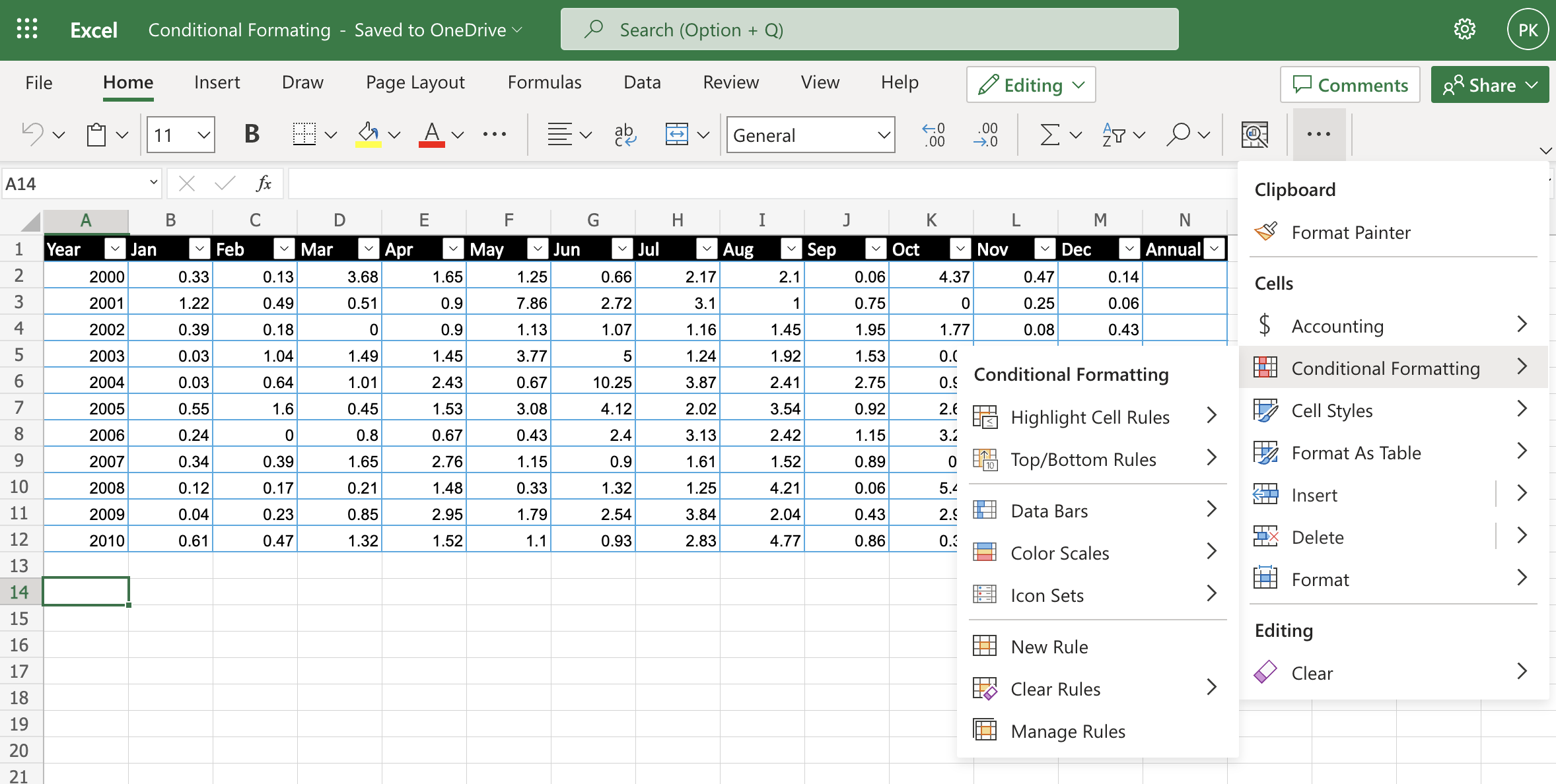
Add data bars to the month columns. This is a really easy way to draw attention to the difference in rainfall between months and years.

• Select all 12 months in all 10 years.
• On the “Home” menu, select Conditional Formatting -> Data Bars -> Green Data Bar in the Gradient Fill section.

The following video shows how to access the Conditional Formatting menu.

Here is a screen shot of the what it should look like when you are done.

Highlight Cells Worksheet

Fill Column N (Annual) in the table using the SUM function.

Set Conditional Formatting for the values in Column N (Annual) to Highlight the cells to have a Red Fill if the annual rainfall is below 16″ and a Green Fill if the annual rainfall is equal to or above 16″.

• Select Conditional Formatting -> Highlight Cell Rules -> Less Than.
• Enter 16 in the last box of the rule.
• In the “format with” drop down, select “light red fill with dark red text” if not all ready selected.
• Click done.
• Click the “plus” sign to add another rule.
• Select greater than or equals to.
• Enter 16 once again.
• In the “format with” drop down, select “green fill with dark green text”
• Click done.

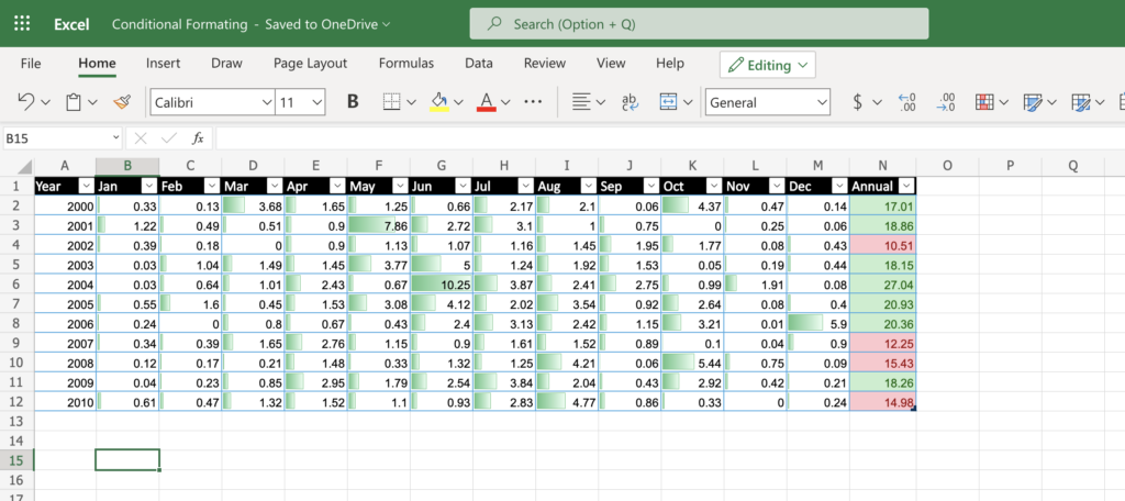
Icon Sets Worksheet

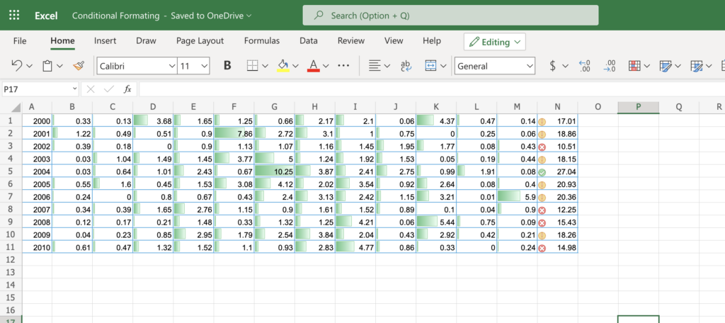
First of all we will clear the formatting from column N (Annual) and replace it with an icon set. Icon sets automatically change based on how an individual cell compares to all the rest. This is a very easy way to emphasize cells that have high or low values.

• Select all ten months in column N (Annual)
• Select Conditional Formatting -> Clear Rules -> Clear Rules from Selected Cells
• With the same cells still selected, Select Conditional Formatting -> Icons Sets.
• Choose one three symbols (Circled) from the Indicators section.
• Still with the same cells selected, Select Conditional Formatting -> Manage Rules.
• Click the little pencil icon to edit the rule.
• Experiment with a few different icon sets. Stop when you feel you have found the icon set that best highlights low, average, and high rain fall years. There is not a right or wrong icon set. It is a matter of what you feel best highlights the information to your audience.

Highlight Text Worksheet

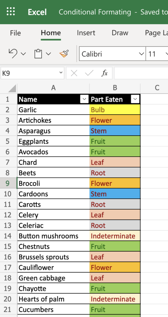
This list shows what part of common fruits and vegetables is eaten. Using what you have learned in the previous exercises, highlight each eatable part with a different background color.

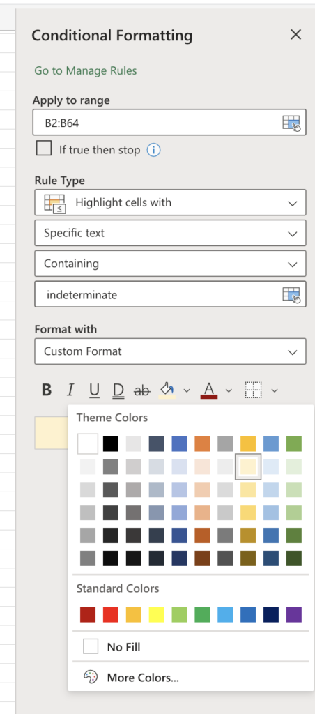
• You will need to start by selecting Conditional Formatting -> Highlight Cell Rules -> Text that contains.
• Experiment with the highlighting options. You may find it best to use a custom fill color. You will find this on the menu of icons below the “format with” drop down.
• Add rules as needed.

Above Average worksheet

In this exercise you will find the average number of chapters in the books of the New Testament. Then you will highlight the book the have more chapters than average.

• Use a Bible to finish filling in the books of the New Testament along with how many chapters each one has.
• Use the AVERAGE function to show the average number of chapters at the bottom of the “# of chapters” column.
• Use the “Conditional Formatting -> Top/Bottom Rules -> Above average” conditional formatting rule to highlight the books that have above average chapters. You can choose which formatting style you think is most appropriate.

Congratulations! Great Work!!