Spanish and English both use the Latin alphabet, but learning your Spanish ABCs is more than just recognizing letters; it’s about getting those sounds just right!
It is easy for English speakers to mix up the pronunciation on Spanish vowels A, I, and E.
If you pronounce papa (potato) as PAY-puh, that’ll sound like pepa (seed) to a Spanish speaker. It may be tempting to pronounce pepa as PEE-puh, a Spanish speaker will think you’re trying to say pipa (pipe).
And that’s just the vowels!
The Spanish alphabet has a total of 27 letters. It includes the same 26 letters as the English alphabet, plus one more: Ñ.
The Spanish alphabet used to have more letters. In 2010, the Real Academia Española decided that the letters CH, LL, and RR should be combined with the letters C, L, and R. As a result, Spanish dictionaries no longer have separate sections for words that begin with those letter pairings.
Just like the English alphabet, the alphabet in Spanish has a name for every letter. When you learned the ABC song as a child, you were singing the names of the English letters. This is so basic that you probably don’t even think about it anymore. In English these names are only spoken and not written. In Spanish the names are written. So you may see them in print. For example, be is the name for the Spanish letter B.
Letter
Name
Example
Pronunciation
Translation
A
a
amigo
ah-MI-goh
friend
B
be (be larga, be alta)
bola
BO-lah
ball
C
ce
casa, cena
KAH-sa, SEN-a
house, dinner
D
de
día
DEE-ah
day
E
e
este
ES-te
this
F
efe
foto
FO-toe
photo
G
ge
gallo, gente
GAH-yo, HEN-te
rooster, people
H
hache
hola
OH-lah
hi
I
i
isla
EEZ-lah
island
J
jota
jefe
HEH-fay
boss
K
ka
kilo
KEE-loh
kilo
L
ele
libro
LEE-bro
book
M
eme
manzana
mahn-ZAH-nah
apple
N
ene
nube
NEW-beh
cloud
Ñ
eñe
niña
NEEN-yah
little girl
O
o
lobo
LO-boh
wolf
P
pe
pato
PAH-toe
duck
Q
cu
queso
KAY-so
cheese
R
erre
radio
RAH-dee-oh
radio
S
ese
sal
SAHL
salt
T
te
tomate
toe-MAH-tay
tomato
U
u
uva
OO-bah
grape
V
ve chica or ve baja
vaca
BAH-kah
cow
W
doble ve, or doble u
wifi
WEE-fee
wifi
X
equis
México
MEH-hee-koh
Mexico
Y
i griega
yo
YOH
I
Z
zeta
zorro
SOU-rroh
fox
A particular letter makes the same sound with very few exceptions. Three exceptions are the letters C, G, and R. These tricky consonants change their pronunciation based on the other letters around them.
The letter C makes a “k” sound when followed by A, O, or U, but it makes an “s” sound (or in Spain, “th” like “thin”) when followed by E or I.
Spanish Word
Pronunciation
Translation
casa
KAH-sah
house
codo
KOH-DOH
elbow
cuna
KUH-nah
cradle
ceja
SAY-ha
eyebrow
cita
SEE-ta
appointment
The letter G makes a hard “g” sound before A, O, or U, but it makes an “h” sound before E or I.
Spanish Word
Pronunciation
Translation
gafas
GAH-fahs
glasses
gota
GOH-ta
drop
gusto
GOOSE-toe
taste, liking, pleasure
gesto
HEHS-toe
gesture
gigante
hee-GAN-tay
giant
The letter R is trilled when at the beginning of a sentence or when it’s a double RR:
Spanish Word
Pronunciation
Translation
recuerdo
rray-KWER-doh
memory
carro
KAH-rroh
car
caro
KAH-roh
expensive
Tongue twisters, or trabalenguas in Spanish, are a fantastic way to work on your pronunciation of the double r.
Erre con erre cigarro, erre con erre barril. (R with R cigar, R with R barrel.)
Rápido corren los carros, sobre los rieles del ferrocarril. (Quickly run the carriages on the rails of the railway.)
We have been working with various tables of data. We learned how to sort data alphabetically and from largest to smallest. This is all very useful and helpful. But what if you want to know the total or some other fact about a portion of the list? Spreadsheets are a great tool for doing exactly that!
Let’s look at a table of data about the 200 largest cities in the United States.
Rank
Name
State
Population 2022
Population 2020
Growth %
Density
Land Area Sq Mi
1
New York City
NY
8930002
8804190
1.41%
29729
300.381
2
Los Angeles
CA
3919973
3898747
0.54%
8359
468.956
3
Chicago
IL
2756546
2746388
0.37%
12124
227.369
4
Houston
TX
2345606
2304580
1.75%
3664
640.194
5
Phoenix
AZ
1640641
1608139
1.98%
3169
517.673
6
Philadelphia
PA
1619355
1603797
0.96%
12060
134.279
7
San Antonio
TX
1456069
1434625
1.47%
3002
485.113
8
San Diego
CA
1402838
1386932
1.13%
4305
325.877
9
Dallas
TX
1325691
1304379
1.61%
3902
339.736
10
San Jose
CA
1026700
1013240
1.31%
5774
177.808
11
Austin
TX
996147
961855
3.44%
3114
319.939
12
Jacksonville
FL
975177
949611
2.62%
1305
747.467
13
Fort Worth
TX
954457
918915
3.72%
2762
345.584
14
Columbus
OH
929492
905748
2.55%
4240
219.197
15
Charlotte
NC
903211
874579
3.17%
2940
307.238
16
Indianapolis
IN
901082
887642
1.49%
2492
361.571
17
San Francisco
CA
887711
873965
1.55%
18927
46.903
18
Seattle
WA
762687
737015
3.37%
9095
83.862
19
Denver
CO
738594
715522
3.12%
4818
153.292
20
Washington
DC
707109
689545
2.48%
11566
61.136
21
Nashville
TN
707091
689447
2.50%
1487
475.543
22
Oklahoma City
OK
701266
681054
2.88%
1156
606.445
23
Boston
MA
687257
675647
1.69%
14217
48.339
24
El Paso
TX
684753
678815
0.87%
2660
257.42
25
Portland
OR
666249
652503
2.06%
4994
133.421
26
Las Vegas
NV
653533
641903
1.78%
4610
141.767
27
Memphis
TN
630348
633104
-0.44%
1986
317.357
28
Detroit
MI
624177
639111
-2.39%
4500
138.715
29
Baltimore
MD
578658
585708
-1.22%
7149
80.947
30
Milwaukee
WI
573700
577222
-0.61%
5965
96.184
31
Albuquerque
NM
568301
564559
0.66%
3036
187.215
32
Fresno
CA
551595
542107
1.72%
4808
114.725
33
Tucson
AZ
547131
542629
0.82%
2299
238.014
34
Sacramento
CA
536635
524943
2.18%
5491
97.73
35
Kansas City
MO
517750
508090
1.87%
1644
314.886
36
Mesa
AZ
517302
504258
2.52%
3746
138.085
37
Atlanta
GA
514457
498715
3.06%
3790
135.737
38
Omaha
NE
501469
486051
3.07%
3557
140.983
39
Colorado Springs
CO
491467
478961
2.54%
2520
195
40
Raleigh
NC
480419
467665
2.65%
3293
145.886
41
Long Beach
CA
467638
466742
0.19%
9224
50.696
42
Virginia Beach
VA
463766
459470
0.93%
1895
244.723
43
Miami
FL
450797
442241
1.90%
12524
35.996
44
Oakland
CA
450630
440646
2.22%
8062
55.893
45
Minneapolis
MN
439430
429954
2.16%
8138
54
46
Tulsa
OK
417298
413066
1.01%
2113
197.478
47
Bakersfield
CA
414649
403455
2.70%
2769
149.758
48
Wichita
KS
400564
397532
0.76%
2478
161.662
49
Arlington
TX
400032
394266
1.44%
4177
95.779
50
Aurora
CO
398497
386261
3.07%
2583
154.272
51
Tampa
FL
394809
384959
2.49%
3463
114.017
52
New Orleans
LA
392031
383997
2.05%
2314
169.434
53
Cleveland
OH
367786
372624
-1.32%
4734
77.694
54
Honolulu
HI
353706
350964
0.78%
5842
60.544
55
Anaheim
CA
348936
346824
0.61%
6934
50.32
56
Louisville
KY
344794
386884
-12.21%
1309
263.434
57
Henderson
NV
329586
317610
3.63%
3107
106.082
58
Lexington
KY
327924
322570
1.63%
1156
283.637
59
Irvine
CA
326730
307670
5.83%
4979
65.619
60
Stockton
CA
326624
320804
1.78%
5254
62.172
61
Orlando
FL
321427
307573
4.31%
2907
110.559
62
Corpus Christi
TX
320393
317863
0.79%
2006
159.703
63
Newark
NJ
318431
311549
2.16%
13189
24.144
64
Riverside
CA
317224
314998
0.70%
3904
81.258
65
St. Paul
MN
316819
311527
1.67%
6095
51.978
66
Cincinnati
OH
311791
309317
0.79%
4006
77.836
67
San Juan
PR
311038
322854
-3.80%
7868
39.533
68
Santa Ana
CA
307367
310227
-0.93%
11234
27.361
69
Greensboro
NC
304909
299035
1.93%
2362
129.068
70
Pittsburgh
PA
302425
302971
-0.18%
5461
55.376
71
Jersey City
NJ
301419
292449
2.98%
20444
14.744
72
St. Louis
MO
298034
301578
-1.19%
4827
61.744
73
Lincoln
NE
297622
291082
2.20%
3093
96.223
74
Durham
NC
294542
283506
3.75%
2625
112.221
75
Anchorage
AK
291131
291247
-0.04%
171
1706.8
76
Plano
TX
290624
285494
1.77%
4054
71.682
77
Chandler
AZ
283959
275987
2.81%
4360
65.124
78
Chula Vista
CA
281801
275487
2.24%
5677
49.641
79
Buffalo
NY
281757
278349
1.21%
6978
40.378
80
Gilbert
AZ
279810
267918
4.25%
4086
68.475
81
Madison
WI
277166
269840
2.64%
3493
79.339
82
Reno
NV
271953
264165
2.86%
2501
108.744
83
North Las Vegas
NV
271641
262527
3.36%
2771
98.015
84
Toledo
OH
267603
270871
-1.22%
3325
80.489
85
Fort Wayne
IN
265926
263886
0.77%
2404
110.636
86
Irving
TX
264762
256684
3.05%
3948
67.06
87
Lubbock
TX
262655
257141
2.10%
1950
134.723
88
St. Petersburg
FL
261016
258308
1.04%
4219
61.864
89
Laredo
TX
259027
255205
1.48%
2450
105.743
90
Chesapeake
VA
254864
249422
2.14%
753
338.51
91
Winston-Salem
NC
253531
249545
1.57%
1912
132.614
92
Glendale
AZ
252645
248325
1.71%
4102
61.592
93
Garland
TX
249846
246018
1.53%
4379
57.06
94
Scottsdale
AZ
246157
241361
1.95%
1338
183.987
95
Arlington
VA
244847
238643
2.53%
9418
25.997
96
Enterprise
NV
244501
221831
9.27%
4782
51.129
97
Boise
ID
241686
235684
2.48%
2888
83.674
98
Santa Clarita
CA
239143
228673
4.38%
3380
70.755
99
Norfolk
VA
237045
238005
-0.40%
4449
53.275
100
Fremont
CA
233788
230504
1.40%
3018
77.465
101
Spokane
WA
233003
228989
1.72%
3389
68.759
102
Richmond
VA
231090
226610
1.94%
3856
59.923
103
Baton Rouge
LA
227066
227470
-0.18%
2627
86.449
104
San Bernardino
CA
224537
222101
1.08%
3615
62.108
105
Tacoma
WA
223536
219346
1.87%
4492
49.759
106
Spring Valley
NV
223037
215597
3.34%
6707
33.253
107
Hialeah
FL
222797
223109
-0.14%
10324
21.581
108
Huntsville
AL
221986
215006
3.14%
1036
214.363
109
Modesto
CA
221924
218464
1.56%
5164
42.977
110
Frisco
TX
217213
200509
7.69%
3188
68.125
111
Des Moines
IA
216273
214133
0.99%
2453
88.18
112
Yonkers
NY
214687
211569
1.45%
11919
18.012
113
Port St. Lucie
FL
212901
204851
3.78%
1786
119.202
114
Moreno Valley
CA
211688
208634
1.44%
4130
51.257
115
Worcester
MA
211612
206518
2.41%
5664
37.36
116
Rochester
NY
211480
211328
0.07%
5913
35.766
117
Fontana
CA
210857
208393
1.17%
4895
43.072
118
Columbus
GA
210330
206922
1.62%
972
216.479
119
Fayetteville
NC
210089
208501
0.76%
1421
147.847
120
Sunrise Manor
NV
208868
205618
1.56%
6258
33.376
121
McKinney
TX
208146
195308
6.17%
3109
66.94
122
Little Rock
AR
204405
202591
0.89%
1703
119.992
123
Augusta
GA
203329
202081
0.61%
673
302.274
124
Oxnard
CA
202895
202063
0.41%
7648
26.528
125
Salt Lake City
UT
202379
199723
1.31%
1828
110.698
126
Amarillo
TX
202333
200393
0.96%
1989
101.744
127
Overland Park
KS
202012
197238
2.36%
2687
75.18
128
Cape Coral
FL
201958
194016
3.93%
1906
105.948
129
Grand Rapids
MI
201093
198917
1.08%
4493
44.756
130
Huntington Beach
CA
200455
198711
0.87%
7423
27.003
131
Sioux Falls
SD
200243
192517
3.86%
2560
78.229
132
Grand Prairie
TX
200240
196100
2.07%
2771
72.255
133
Montgomery
AL
199571
200603
-0.52%
1248
159.882
134
Tallahassee
FL
199127
196169
1.49%
1982
100.474
135
Birmingham
AL
198433
200733
-1.16%
1358
146.076
136
Peoria
AZ
198369
190985
3.72%
1127
175.989
137
Glendale
CA
197507
196543
0.49%
6482
30.471
138
Vancouver
WA
196739
190915
2.96%
4036
48.744
139
Providence
RI
193512
190934
1.33%
10514
18.406
140
Knoxville
TN
193114
190740
1.23%
1956
98.713
141
Brownsville
TX
189082
186738
1.24%
1429
132.322
142
Akron
OH
188741
190469
-0.92%
3048
61.933
143
Newport News
VA
187353
186247
0.59%
2716
68.992
144
Fort Lauderdale
FL
186208
182760
1.85%
5384
34.586
145
Mobile
AL
185427
187041
-0.87%
1330
139.465
146
Shreveport
LA
185249
187593
-1.27%
1725
107.361
147
Paradise
NV
184852
191238
-3.45%
3956
46.732
148
Tempe
AZ
184361
180587
2.05%
4612
39.977
149
Chattanooga
TN
183783
181099
1.46%
1286
142.963
150
Cary
NC
182619
174721
4.32%
3110
58.725
151
Eugene
OR
180748
176654
2.27%
4095
44.138
152
Elk Grove
CA
180746
176124
2.56%
4300
42.033
153
Santa Rosa
CA
180189
178127
1.14%
4238
42.519
154
Salem
OR
179715
175535
2.33%
3691
48.691
155
Ontario
CA
177533
175265
1.28%
3553
49.963
156
Aurora
IL
177070
180542
-1.96%
3934
45.009
157
Lancaster
CA
176892
173516
1.91%
1876
94.281
158
Rancho Cucamonga
CA
176289
174453
1.04%
4394
40.117
159
Oceanside
CA
175464
174068
0.80%
4253
41.256
160
Fort Collins
CO
174974
169810
2.95%
3060
57.182
161
Pembroke Pines
FL
174464
171178
1.88%
5340
32.673
162
Clarksville
TN
173480
166722
3.90%
1756
98.796
163
Palmdale
CA
172790
169450
1.93%
1629
106.076
164
Garden Grove
CA
172163
171949
0.12%
9588
17.957
165
Springfield
MO
171112
169176
1.13%
2077
82.392
166
Hayward
CA
166708
162954
2.25%
3661
45.537
167
Salinas
CA
166162
163542
1.58%
7092
23.428
168
Alexandria
VA
163367
159467
2.39%
10939
14.934
169
Paterson
NJ
162438
159732
1.67%
19308
8.413
170
Murfreesboro
TN
161571
152769
5.45%
2618
61.709
171
Bayamon
PR
161242
165368
-2.56%
5977
26.978
172
Sunnyvale
CA
158949
155805
1.98%
7215
22.03
173
Kansas City
KS
158771
156607
1.36%
1272
124.815
174
Lakewood
CO
158584
155984
1.64%
3684
43.047
175
Killeen
TX
158129
153095
3.18%
2899
54.545
176
Corona
CA
158088
157136
0.60%
3954
39.986
177
Bellevue
WA
157752
151854
3.74%
4715
33.461
178
Springfield
MA
156503
155929
0.37%
4911
31.869
179
Charleston
SC
156255
150227
3.86%
1413
110.554
180
Hollywood
FL
155527
153067
1.58%
5703
27.269
181
Roseville
CA
153569
147773
3.77%
3484
44.079
182
Pasadena
TX
152532
151950
0.38%
3500
43.586
183
Escondido
CA
152464
151038
0.94%
4086
37.314
184
Pomona
CA
152245
151713
0.35%
6625
22.982
185
Mesquite
TX
152164
150108
1.35%
3220
47.252
186
Naperville
IL
151078
149540
1.02%
3893
38.811
187
Joliet
IL
150948
150362
0.39%
2353
64.152
188
Savannah
GA
150078
147780
1.53%
1444
103.91
189
Jackson
MS
149739
153701
-2.65%
1348
111.086
190
Bridgeport
CT
149538
148654
0.59%
9309
16.064
191
Syracuse
NY
149310
148620
0.46%
5965
25.03
192
Surprise
AZ
148274
143148
3.46%
1372
108.063
193
Rockford
IL
147811
148655
-0.57%
2296
64.379
194
Torrance
CA
147393
147067
0.22%
7183
20.521
195
Thornton
CO
146487
141867
3.15%
4081
35.891
196
Kent
WA
145424
136588
6.08%
4309
33.75
197
Fullerton
CA
145309
143617
1.16%
6478
22.431
198
Denton
TX
145167
139869
3.65%
1508
96.236
199
Visalia
CA
144772
141384
2.34%
3817
37.924
200
McAllen
TX
144676
142210
1.70%
2202
65.698
You already know how to use the SUM() function to find the total of a range of cells. So you could easily find the total land area for all 200 cites. Or the total of any of the other columns. But let’s learn a very useful way to find the totals for individual states.
Create a new file
Let’s copy the table into a new spreadsheet file.
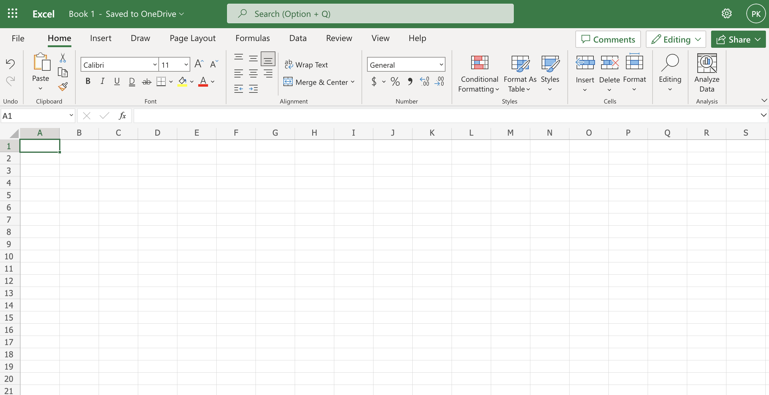
Start from the main office.com screen and click on the Excel icon
Then click on “New blank workbook”
In the green bar along the top, click on the default file name and rename it to “Filter and Subtotal”
Then copy the data from the table of information about the cities.
Paste it into your new worksheet.
Click on the little dialog that is usually on the right side towards the bottom and then choose “Paste Values”. This will remove the formatting from this web page and just pasted the plain values into the spreadsheet.
The easiest way to fix the column width is click on the upper left square of the grid to select all the rows and columns. Then double click the line between two columns and all the columns should autoresize to fit the information inside. If just the data is selected like it will be after you paste it in, it won’t work correctly. You need to select all the column as described.
If you like, you can give the sheet a better name by double clicking on the tab where it says “Sheet1” and giving it a more descriptive name.
If you need help, watch the video on the “Sorting” lesson.
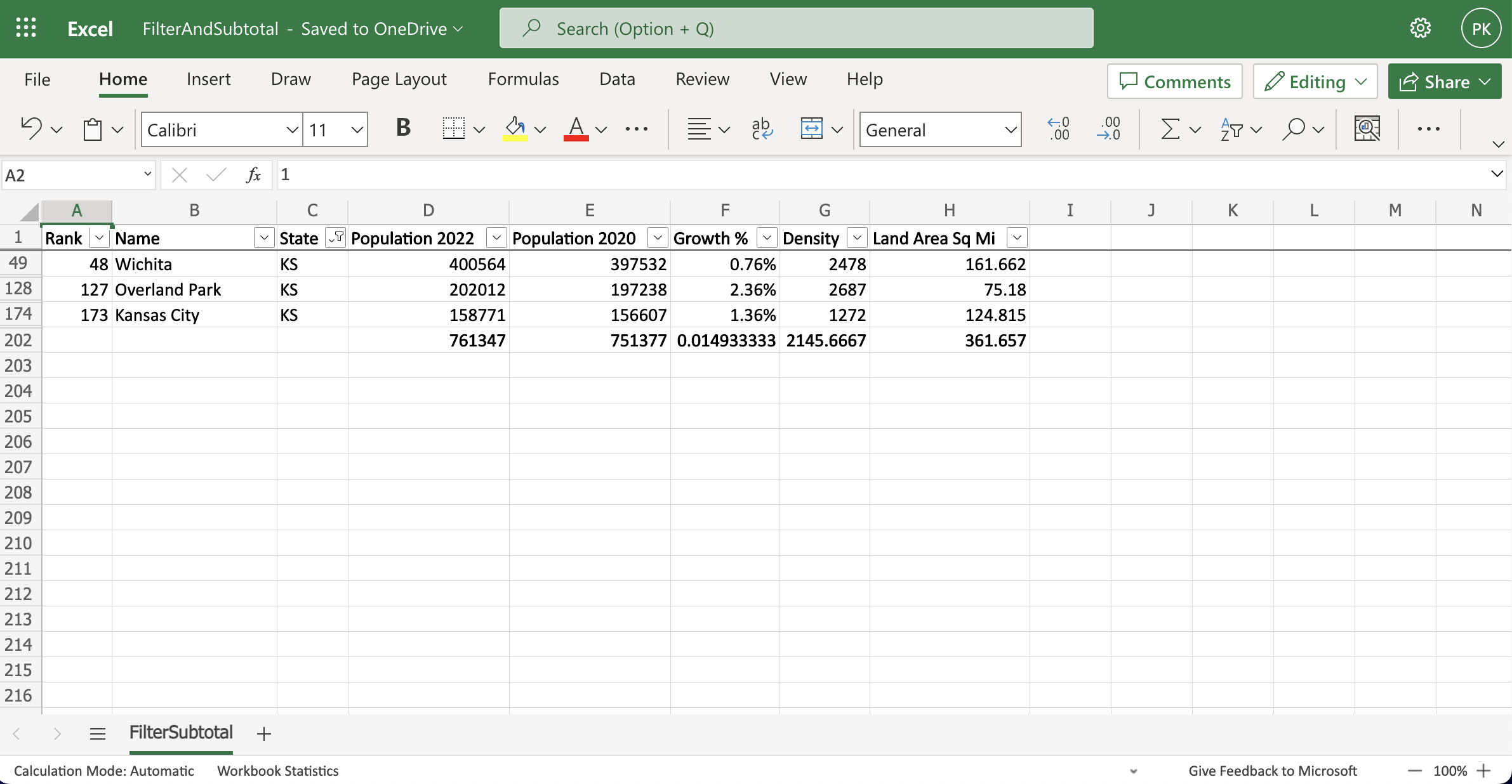
Find a subtotal (the hard way)
Let’s find the total land area for the just cities in KS. This is often referred to as a subtotal. This is because it is a total of a subset, or portion, of the data.
First of all we can do it using ways we have already learned.
Sort the table by state. Refer the the “Sorting” lesson if needed
Add a SUM() function on the bottom of the “Land Area” column. Choose the three KS cities for your range value in the SUM() function. All three cities should be together because you sorted the table by state. Your formula should look something like this: =SUM(H94:H96).
Ok! Did you get a total of 361.657? If so, that worked great!
However, you will notice that this method requires you to manually change the range that you sum if you want to change which state you are analyzing. It’s just not as convenient as it could be.
If you re-sort the list by a different column you will notice a different problem. Try sorting by “name”. What happens to the total land area? It’s not totaling the Kansas cities anymore. It is still totaling the cells you asked it to but the cities from KS are no longer there.
So let’s learn a better way. First we will undo what we just did. Then we’ll learn how to filter the data to just show the part we are interested in. And then we’ll learn to use SUBTOTAL().
Undo your changes
Let’s get the table of data back to how it originally was. There are two methods of doing this. You can try whichever way you would like.
Method #1 – Using undo
On the “Home” menu ribbon, press the undo button enough times to undo everything your previous changes and return it to how it was right after you pasted the data into the sheet.
Method #2 – Manually change it back to how it was.
Sort the table by “rank” smallest to largest.
Delete the formula in the cell where you entered the SUM() function.
Filtering
All the major spreadsheet applications can selectively hide and show data. This is called filtering. Only data that matches the filter passes though and is shown. The data that does not match the filter is hidden. It is not deleted, only hidden, and will reappear when the filter is removed.
OK, time to practice!
Click on the “Data” menu ribbon if you are not already there.
Select a cell within the table of data
Click the filter button
Notice the dropdown arrows by each column heading
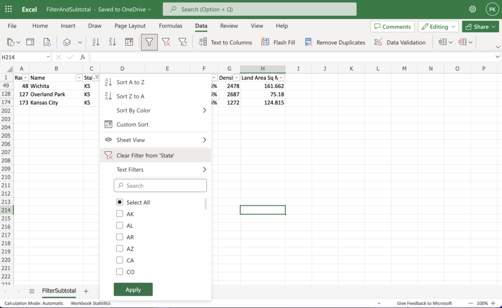
Click on the drop down for “State”
Uncheck the “select all” box
Scroll down as needed and select the checkbox for KS
Click apply
Watch the video if you need help.
Note how the row numbers for the hidden data are missing. They are hidden along with the data. The rows that are shown, in this case the rows with KS in the state column, retain their original row numbers.
Ok now remove the filter.
Click on the filter/dropdown arrow in the header of the “State” column
Click on Clear Filter from ‘State’
Remove Filter
Make the table a little nicer
Before we move on, let do a couple of things that will make it easier to use the table
Select the top row and apply bold formatting.
Select the entire sheet and double click on a column border to auto expand them to the correct width.
Click on the “View” ribbon and then click Freeze Panes -> Freeze Top Row
Watch the video if you need help.
Experiment with SUM() before learning about SUBTOTAL()
Now let’s experiment with the SUM() function. How does it work with filtered/hidden data?
Add a SUM() function with the correct range at the bottom of the data in the “Land Area” column. This will likely be something like: =SUM(H2:H201)
Click on the dropdown on the “State” column header again.
Select a state of your choice.
Was the total hidden along with the other rows? Excel tends to hide the next couple of rows on the bottom of the data along with the other rows.
To see everything again, remove the filter again.
Enter a SUM() function three or more rows below the data.
Try filtering the “State” column again.
Observe the total below the “Land Area” column. It should not be hidden this time. Notice that it doesn’t change. That is because all the rows are still there. We noticed earlier that the row numbers are missing when rows are hidden. They are hidden but still exist so the SUM() function is doing exactly what we told it to do. It is adding all the rows together in your range regardless if they are hidden or not.
In this case, this isn’t what we want to happen. We want to know the total for just the filtered rows. SUBTOTAL() works really well for this.
Using SUBTOTAL()
This function is quite flexible and useful. It can be used to find the total, or the average, or smallest, or the largest, and a number of other things in a column of numbers.
Let’s jump right in.
Enter a SUBTOTAL() function right below the data in the “Population 2022” column. You don’t need to worry about putting it three rows down. Excel will not hide this formula.
SUBTOTAL() takes two pieces of information. The type of calculation you want to do. And the range on which you wish to perform the calculation.
As you start to type in the function you will see a link for more information. Click on this to see what number you should use to sum the range and ignore the hidden rows. You will see that you need to use 109.
Then enter the range.
When you are finished your formula should look like this: =SUBTOTAL(109,D2:D201)
Now you can filter by any state you wish and the subtotal will show you the population for just the filtered cities!
This may be a lot easier to follow by watching the video.
Adding a Subtotal
Congratulations! Now you know how to find the subtotal for filtered information.
To finish up:
Add a subtotal to the “Population 2020” column just like you did on the “Population 2022” column.
Do the same on the “Land Area” column. Delete the SUM() you did earlier if you haven’t already done so.
On the “Growth %” and “Density” columns add a subtotal for the average. You will need to click on the more information link to see which number to use.
Format the bottom row of totals bold so they stand out a little more.
When you are finished it should look a lot like the photo at the top of this lesson. In the photo the data has been filtered to just show cities in KS.
People have worked with lists and tables of data for centuries. Until the last few decades the only option was a hand written list. You can imagine that a hand written list of information is not easily rearranged!
Let’s say you wrote down a list of names of people to invite to a reunion. You wrote the list in order by first name. Then you realize that you would prefer it in order by last name. So now you will need to write the list all over again in the correct order.
If you had typed it in an application like Microsoft Word or Google Docs it would be somewhat easier. You could copy and paste to move each line to where it belongs. But that still is tedious and takes a lot of time.
There is a better easier way! Spreadsheets are great at sorting data.
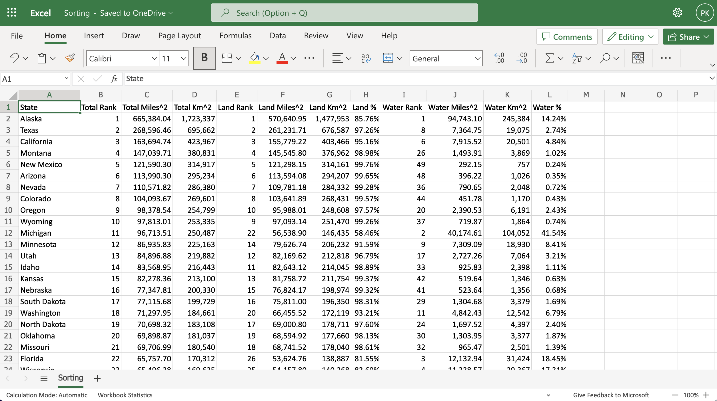
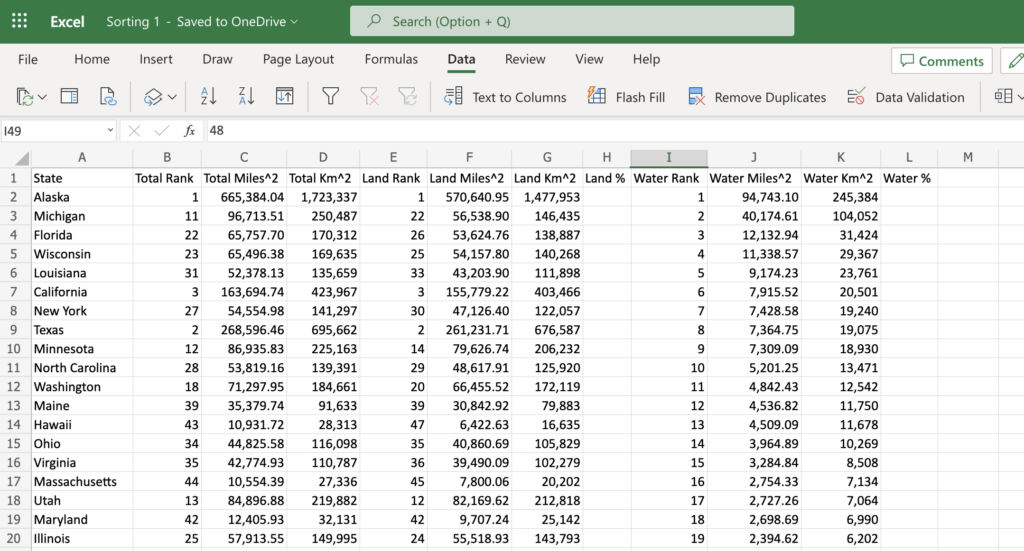
Take a look at the follow in table of information about the fifty states of the USA. It looks like it is sorted by total square miles right now. But what if you wanted to see it in order by square miles of water? How about alphabetically by state name? How many ways could the data be arranged?
State
Total Rank
Total Miles^2
Total Km^2
Land Rank
Land Miles^2
Land Km^2
Land %
Water Rank
Water Miles^2
Water Km^2
Water %
Alaska
665,384.04
1,723,337
570,640.95
1,477,953
94,743.10
245,384
Texas
268,596.46
695,662
261,231.71
676,587
7,364.75
19,075
California
163,694.74
423,967
155,779.22
403,466
7,915.52
20,501
Montana
147,039.71
380,831
145,545.80
376,962
1,493.91
3,869
New Mexico
121,590.30
314,917
121,298.15
314,161
292.15
757
Arizona
113,990.30
295,234
113,594.08
294,207
396.22
1,026
Nevada
110,571.82
286,380
109,781.18
284,332
790.65
2,048
Colorado
104,093.67
269,601
103,641.89
268,431
451.78
1,170
Wyoming
97,813.01
253,335
97,093.14
251,470
719.87
1,864
Oregon
98,378.54
254,799
95,988.01
248,608
2,390.53
6,191
Idaho
83,568.95
216,443
82,643.12
214,045
925.83
2,398
Utah
84,896.88
219,882
82,169.62
212,818
2,727.26
7,064
Kansas
82,278.36
213,100
81,758.72
211,754
519.64
1,346
Minnesota
86,935.83
225,163
79,626.74
206,232
7,309.09
18,930
Nebraska
77,347.81
200,330
76,824.17
198,974
523.64
1,356
South Dakota
77,115.68
199,729
75,811.00
196,350
1,304.68
3,379
North Dakota
70,698.32
183,108
69,000.80
178,711
1,697.52
4,397
Missouri
69,706.99
180,540
68,741.52
178,040
965.47
2,501
Oklahoma
69,898.87
181,037
68,594.92
177,660
1,303.95
3,377
Washington
71,297.95
184,661
66,455.52
172,119
4,842.43
12,542
Georgia
59,425.15
153,910
57,513.49
148,959
1,911.66
4,951
Michigan
96,713.51
250,487
56,538.90
146,435
40,174.61
104,052
Iowa
56,272.81
145,746
55,857.13
144,669
415.68
1,077
Illinois
57,913.55
149,995
55,518.93
143,793
2,394.62
6,202
Wisconsin
65,496.38
169,635
54,157.80
140,268
11,338.57
29,367
Florida
65,757.70
170,312
53,624.76
138,887
12,132.94
31,424
Arkansas
53,178.55
137,732
52,035.48
134,771
1,143.07
2,961
Alabama
52,420.07
135,767
50,645.33
131,171
1,774.74
4,597
North Carolina
53,819.16
139,391
48,617.91
125,920
5,201.25
13,471
New York
54,554.98
141,297
47,126.40
122,057
7,428.58
19,240
Mississippi
48,431.78
125,438
46,923.27
121,531
1,508.51
3,907
Pennsylvania
46,054.34
119,280
44,742.70
115,883
1,311.64
3,397
Louisiana
52,378.13
135,659
43,203.90
111,898
9,174.23
23,761
Tennessee
42,144.25
109,153
41,234.90
106,798
909.36
2,355
Ohio
44,825.58
116,098
40,860.69
105,829
3,964.89
10,269
Virginia
42,774.93
110,787
39,490.09
102,279
3,284.84
8,508
Kentucky
40,407.80
104,656
39,486.34
102,269
921.46
2,387
Indiana
36,419.55
94,326
35,826.11
92,789
593.44
1,537
Maine
35,379.74
91,633
30,842.92
79,883
4,536.82
11,750
South Carolina
32,020.49
82,933
30,060.70
77,857
1,959.79
5,076
West Virginia
24,230.04
62,756
24,038.21
62,259
191.83
497
Maryland
12,405.93
32,131
9,707.24
25,142
2,698.69
6,990
Vermont
9,616.36
24,906
9,216.66
23,871
399.71
1,035
New Hampshire
9,349.16
24,214
8,952.65
23,187
396.51
1,027
Massachusetts
10,554.39
27,336
7,800.06
20,202
2,754.33
7,134
New Jersey
8,722.58
22,591
7,354.22
19,047
1,368.36
3,544
Hawaii
10,931.72
28,313
6,422.63
16,635
4,509.09
11,678
Connecticut
5,543.41
14,357
4,842.36
12,542
701.06
1,816
Delaware
2,488.72
6,446
1,948.54
5,047
540.18
1,399
Rhode Island
1,544.89
4,001
1,033.81
2,678
511.07
1,324
Create a new file
Let’s copy the table into a new spreadsheet file.
Start from the main office.com screen and click on the Excel icon
Then click on “New blank workbook”
In the green bar along the top, click on the default file name and rename it to “sorting”
Then copy the data from the table of information about the states.
Paste it into your new worksheet.
Click on the little dialog that is usually on the right side towards the bottom and then choose “Paste Values”. This will remove the formatting from this web page and just pasted the plain values into the spreadsheet.
The easiest way to fix the column width is click on the upper left square of the grid to select all the rows and columns. Then double click the line between two columns and all the columns should autoresize to fit the information inside. If just the data is selected like it will be after you paste it in, it won’t work correctly. You need to select all the column as described.
If you like, you can give the sheet a better name by double clicking on the tab where it says “Sheet1” and giving it a more descriptive name.
If you need help, watch the following video.
Create new workbook for sorting
Now you are ready to sort the information.
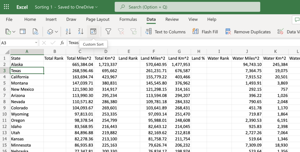
Click the “Data” menu.
Select a cell somewhere within the table of data if you haven’t already.
Click the “Custom Sort” icon
Custom Sort
In the custom sort dialog, select “State” for the column.
Leave the default sort on “Cell Values”.
Also leave it on “Sort Ascending”.
Click OK
Now the list should be sorted by “State”!
Auto Fill
All the major spreadsheets, including Excel, make it very easy to auto fill values from example content that shows a pattern. We’ll use this capability to add ranking numbers to the Total Miles^2, Land Miles^2, and Water Miles^2.
Re-sort the list to be sorted by the Total Miles^2 in descending order.
Type a “1” in “B2” and “2” in “B3”. This establishes a pattern of incrementing by 1.
Select both cells
Now click the handle on the bottom right corner of the selected cells and drag the selection down to the bottom of the data.
Watch the follow video if you have any questions.
Auto Fill
That was really easy!
Now experiment with different patterns.
Enter a “5” in “B2” and a “10” in “B3”
Select both cells and then use the handle to auto fill down like you did before.
Note how it counts up by 5s!
Ok, now change it back to count up by 1s.
Continue Sorting and Ranking
Now sort and rank the “Total Land Miles^2” and “Total Water Miles^2.
If you want to try a quicker way, you can sort the table by having a cell selected in the column that you want to sort. Then clicking either the “Sort Ascending” or “Sort Descending” icons that are to the left of the “Custom Sort” icon.
Does your worksheet look like the following screenshot? If not, see if you can fix it.
Sorting Completed
Add Some Data
Now let’s add in the percent of land and water information. Don’t worry! It’s not hard.
Enter your first formula for the percent of land in “H2”.
Remember how to figure what percent a part is of the total? Just divide the part by the total. Or in other words “Total Land Miles^2 / Total Miles^2.
What are the cells that we need to use? Try “=F2/C2”.
Now copy the formula down to the bottom of the data.
Since it is showing is as a decimal we need to format the column as percentage.
Select the entire “H” column by clicking the H.
Go to the “Home” menu.
Now choose the correct format of “Percentage” from the drop down list.
Format Column
OK! Now do the same for the “Water %” column.
Enter the formula.
Copy/Drag it down.
Re-format it to “Percentage”.
Now you can sort the data by any column that you wish!!
The world is full of data. It always has been. For millennium people have needed to organize and record information. That information was then used in many different ways.
The Bible is a very interesting source of examples of early data collection and manipulation.
Joseph taking care of Potifer’s house.
The Parable of the Unjust Steward
All the record keeping in the book of Numbers
In current times the amount of data is more than every because electronic devices allow us as mankind to collect and store data as never before. Fortunately, we also have excellent electronic tools to manipulate all this data. One of the most common and useful of these tools is a spreadsheet.
Spreadsheets
Spreadsheets are electronic applications for storing and working with data. They work especially well with information that is organized in tables of rows and columns. Information arranged this way is often called tabular data.
The term spreadsheet also refers to an electronic document that is created and edited by a spreadsheet application.
These document are structured in row and columns. Columns are named with letters of the alphabet. Rows are identified with numbers. Each individual location in the document is called a “cell”. The default name of a cell is the the name of the column and row it which it is located.
A
B
C
D
E
1
Column/Row
Row
Row
Row
Row
2
Column
3
Column
C3
4
Column
Spreadsheet Column and Row names
As you can see, cell “C3” is so named because it is located at the intersection of column “C” and row “3”.
Most all spreadsheet applications share common features and abilities.
A spreadsheet stores information. Each cell may contain either numbers, text, or the results of formulas that automatically calculate and display a value based on the contents of other cells.
A spreadsheet has many formulas for doing mathematical operations, financial calculations, manipulating text, as well as more complex things like checking if certain criteria is met or not.
A spreadsheet can sort long lists of data. For example, a long list that has names in column “A” and birthdates in column “B” could be sorted by column “B” from youngest to oldest. It doesn’t matter in what order they were originally entered.
A spreadsheet can also filter rows of information to show only rows that meet your criteria and hide all the other rows. In a list of vehicle makes and models, all the Toyota models could be shown and all the other models from every other make could be hidden.
Information can be highlighted with different colors or fonts when it meets criteria that you define. For example, in a column of dollar amounts, every cell over $100 could be highlighted in green. All the cells with $100 or less could be highlighted in red. This is called conditional formatting.
Spreadsheets can summarize data in an easy to understand way by using charts.
This is a short list of basic features. Spreadsheets are capable of doing many more things!
Early Spreadsheet Applications
Many spreadsheet applications have come and gone. VisiCalc is one of them. It was first available for the Apple II in 1979 and then the IBM PC in 1981. While VisiCalc was not the first spreadsheet application, it was an early one that really helped the spreadsheet concept become popular.
Just a few years later Lotus 1-2-3, along with its competitor Borland Quattro, became even more popular than VisiCalc.
Microsoft released the first version of Excel for the Macintosh on September 30, 1985, and then ported it to Windows. By 1995, Excel was the market leader, edging out Lotus 1-2-3.
Modern Spreadsheet Applications
There are a number of modern spreadsheet applications. The most popular ones include:
Microsoft Excel – There are versions for PC, Mac, and the web
Google Sheets – Web based
Numbers for iOS
LibreOffice Calc – available for numerous operating systems
The concepts you will learn in these lessons can be used in any of the modern spreadsheet applications. There are differences in the menus and other parts of the user interfaces. But all of them are fully capable of doing the things mentioned in this lesson.
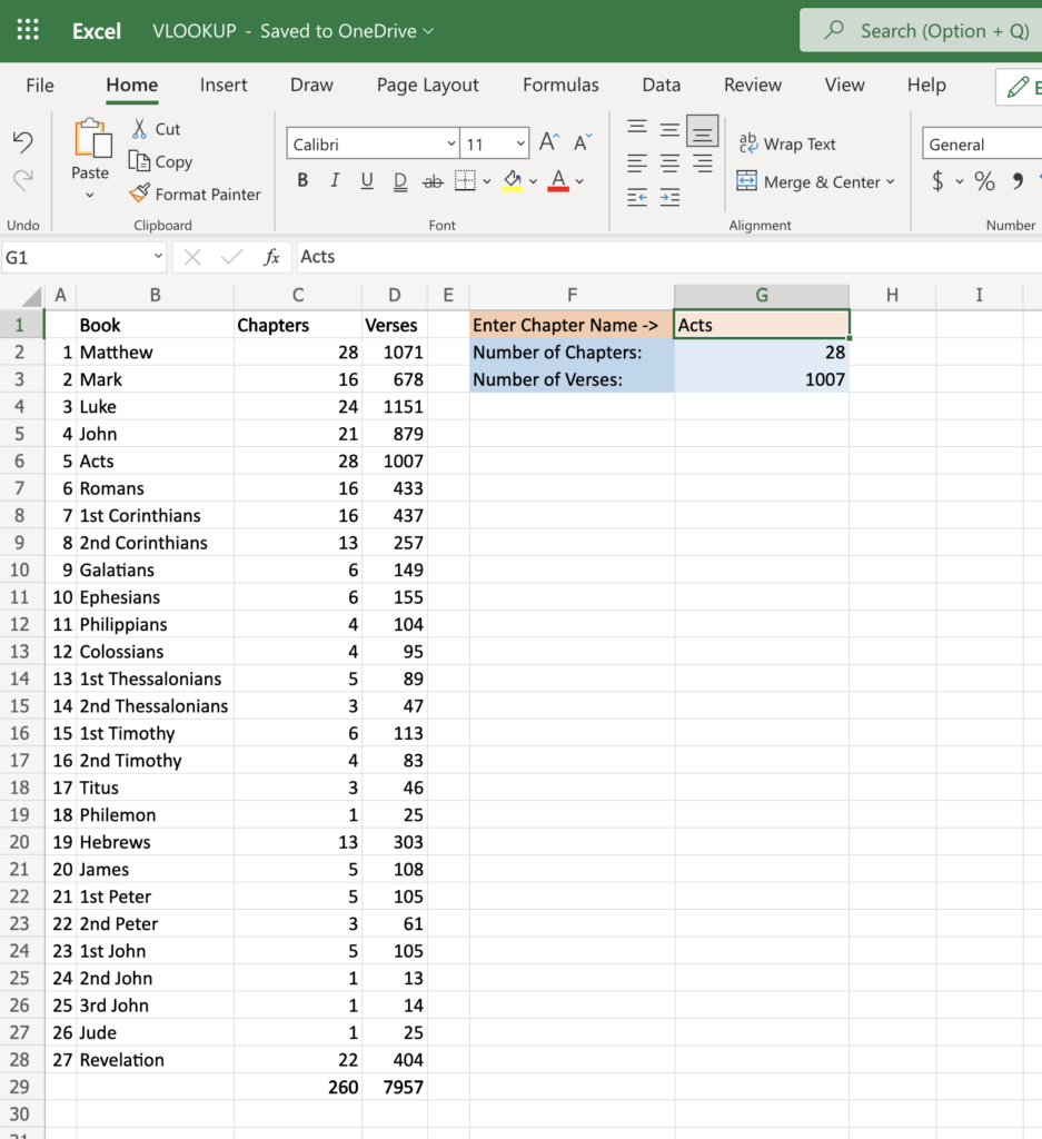
VLOOKUP stands for “Vertical Lookup”. It is a function that makes Excel search for a certain value in a column, the “table array”, in order to return a value from a different column in the same row.
From the main office.com screen, upload the file from your download folder.
VLOOKUP() False Worksheet
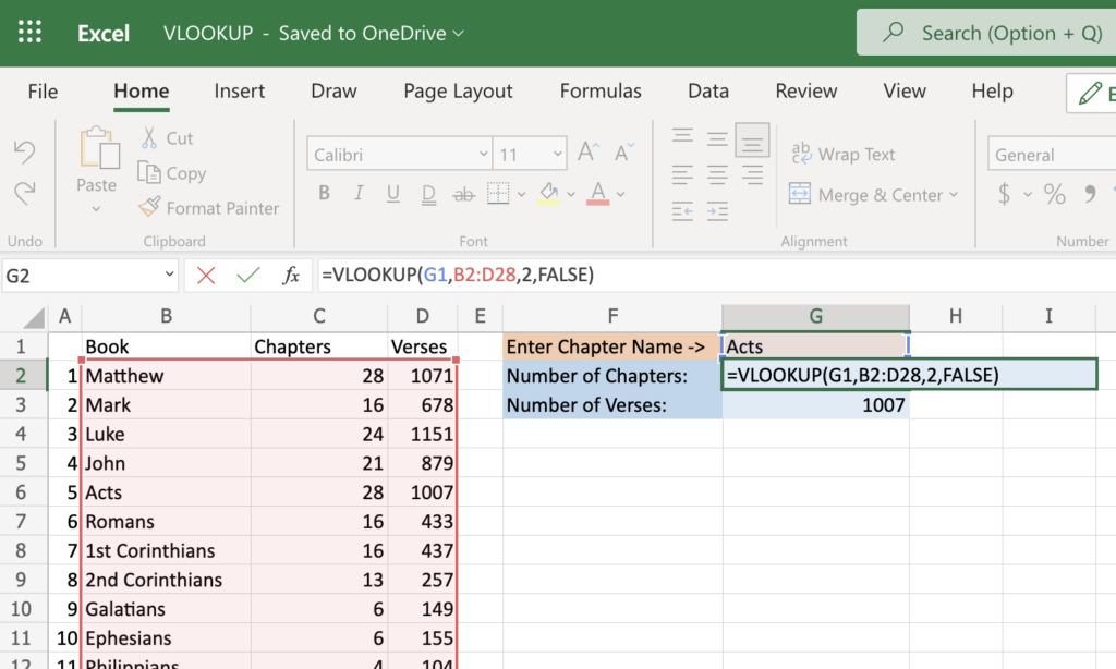
Start by entering a VLOOKUP() function in G2.
The VLOOKUP() function has 4 components. Use the Following screen shot for reference.
VLOOKUP() False
#1 – First is the value you want to look up. In this example we are giving VLOOKUP() the book name from G1.
#2 – The range in which you want to find the value and the return value. This is B2:D28. VLOOKUP() always searches in the leftmost column of the range. In our example this is column B or the column containing the book names. Note: The column you want to search needs to be to the left of the column that has the information you want to return. If it isn’t, you will need to rearrange the columns so that it is. In our case it is already on the left so we don’t need to move any columns.
#3 – The number of the column within your defined range that contains the return value. In our case is the “Chapters” column or column C. We have to tell VLOOKUP to get the answer from column 2. This is because it is the 2nd column in the range we gave VLOOKUP() in the last step.
#4 – We will enter “FALSE” 0 or FALSE tells VLOOKUP() that we want an exact match with the value you are looking for. 1 or TRUE tells VLOOKUP() to look for an approximate match. When working with text you will almost always use FALSE for exact match.
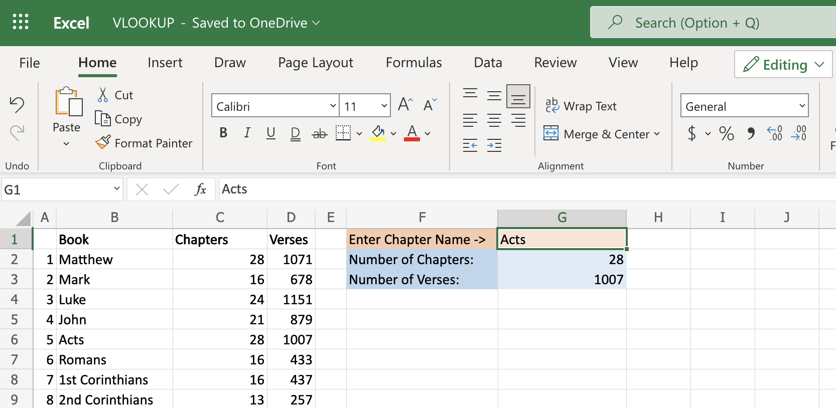
OK! Now you should be able to enter a book of the New Testament in G1 and get the number of chapters back in G2.
Now write a formula in G3 that will display the number of verses. It will be very similar to the formula you just wrote. But the column number will be different.
Enter different books into the G1 cell and watch the “Number of Chapters” and “Number of Verses” change!
To make your information even more interesting, add totals using the SUM() function at the bottom of columns C and D. This will tell us how many chapters and verses are in the New Testament.
Another thing you can do to make the data look better is make the top row bold. Simply select the cell across the top of the table of data and then click the bold button on the “Home” menu.
Go ahead and make the totals bold as well.
Here is a screenshot of the completed worksheet.
Completed Worksheet
VLOOKUP() True Worksheet
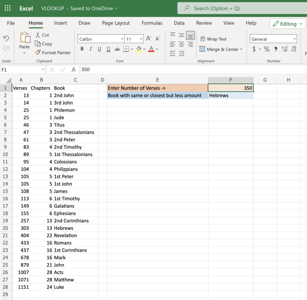
It is possible to use VLOOKUP() to find a close match. That is what the “True” setting is for. This is most useful when searching for numbers.
The data needs to be in the correct order for this to work correctly. Just like before, the column you want to search for a match need to be the leftmost of the range.
Additionally the data in the column you are searching need to be sorted ascending. This is because VLOOKUP() goes down the column looking for a match. If it doesn’t find an exact match, it goes until it finds a value that is larger the the one it is looking for. It then stops and returned the previous value. In other words it returns the value that is closed to what you are searching for but is smaller. There could possibly be a value that is even closer to the target. But if it is larger than the searched for value it will not be returned. The returned answer will always be exactly the same or smaller than the search value.
You don’t need to worry about sorting this data though. It is already sorted correctly.
OK, let’s give it a try!
Start by typing your formula into cell F2
Enter: “=VLOOKUP(F1” This tells VLOOKUP() to search for data that match what is in cell F1
Type a comma and continue with the range: =VLOOKUP(F1,A2:C28
Now another comma and enter the row number that has the answer you want to return.
One more comma and then enter True and then the closing parenthesis.
Does your worksheet look like this?
VLOOKUP() True
Experiment with entering different numbers in cell F1.
If you enter a number that is exactly what a book has it should return the name of that book.
If you enter a number that is not in the list it should find the closest one that is smaller.
In this lesson we will work with some more functions.
LEFT() and RIGHT() are some useful functions for separating out a part text that exists inside of a larger string of text.
We can also use CONCAT() to join multiple cells into one string of text.
If we want to check for multiple things to select a part of our data we might need functions like AND() and OR().
What can we do if we want to count or add up just a portion of our data that meets a certain criteria? The COUNTIF() and SUMIF() functions can help us out!
From the main office.com screen, upload the file from your download folder.
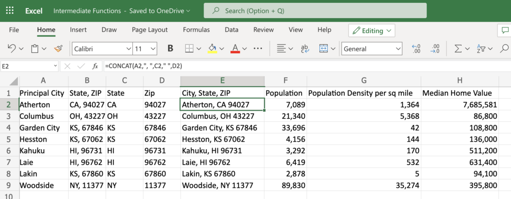
LEFT(), RIGHT() and CONCAT() worksheet
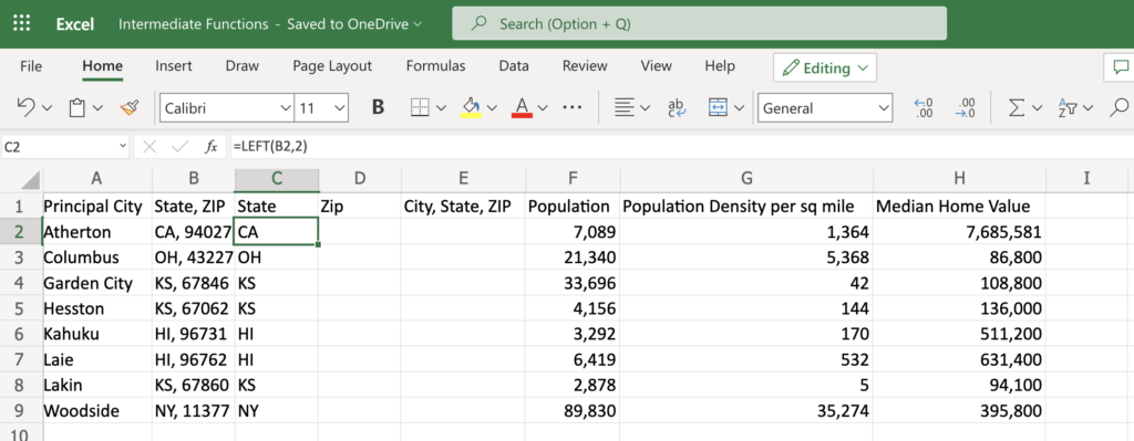
Both the LEFT() and RIGHT() functions extract the number of characters that you ask for from a cell reference. Their names indicate from which end of the text they start.
Try extracting the state abbreviation from B2.
Start entering the formula in C2 because that is where you want the information to end up.
Use LEFT() to start extracting from the left side. So start with =LEFT(
Then enter the cell from which you want to extract the characters. =LEFT(B2,
Now tell the function how many characters you want. =LEFT(B2,2)
Great! Now copy the formula down to the bottom of the data.
This is how it should look.
RIGHT() Function
Now extract the ZIP code from B2 into D2.
You will need to use the RIGHT() function
Don’t forget to ask for 5 characters. Note that this function works from the right and counts to the left.
Copy the formula down to the bottom of the data.
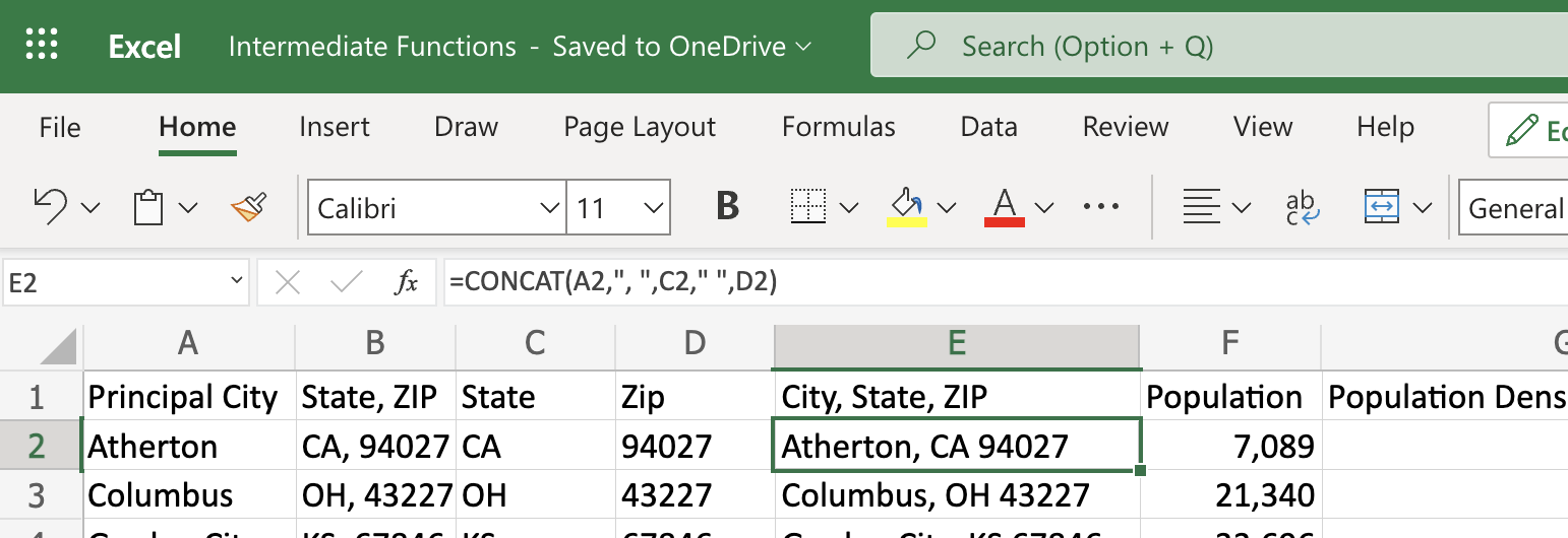
Not only is it easy to separate information out, it is also easy to join information together!
Let’s joint or concatenate the City together with the State and ZIP.
Start by entering your formula in row 2 of column E (City, State, ZIP)
You need to give the CONCAT() function all the items you want it to put together. Separate each one with a comma. Like this: =CONCAT(A2,C2,D2)
What’s wrong? Is everything all ran together? That is because we have to explicitly tell the CONCAT() function where we want commas and spaces.
Try adding a comma and space between the City and State. You will need to put any text that doesn’t come from a cell reference inside quotes. Like this: =CONCAT(A2,”, “,C2,D2). That is how the CONCAT() function can tell the difference between when you are using a comma to separate values and when you want it to include the comma in the joined text.
Now add just a space between the State and ZIP!
Here is what the worksheet should look like now.
CONCAT() Function
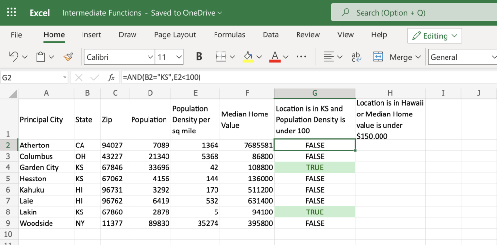
AND() and OR() Worksheet
Sometimes you will need to identify data by multiple criteria. Maybe two or three things need to be true about the data before it meets your criteria. It could also be that if any of serveral things are true it would meet your criteria. This is exactly what the AND() and OR() functions are for!
To use either function you give them a list of logical test separated by commas.
The AND() function finds FEWER results the more criteria or logical test you give it. This is because the all have to be true. Hence the name. Criteria one needs to be met AND criteria two and so forth.
The OR() function is very different. It finds MORE results the more criteria you give it. Once again the name explains how it works. If logical test one OR logical test two is true then it accepts it as correct.
Both of these functions display their findings as true or false.
Let’s get started.
In G2 build a formula with that checks if the State=KS and that the population density<100.
The logical tests are separated by a comma so it will be: =AND(B2=”KS”, ??) Where the question marks are you will need to enter the second logical test.
Copy the formula down to the bottom of the data.
Do you remember how to highlight cell with conditional formatting? Review that lesson if needed. Then hight light all the cell that say “TRUE” with green.
The result should look like this.
AND() Function
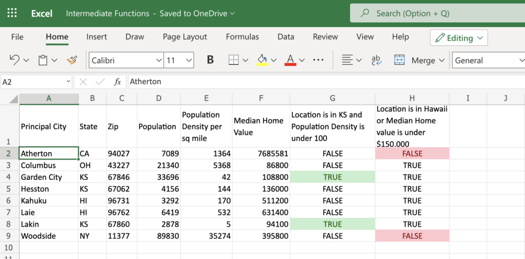
Now let’s find rows where either of two test are true. Maybe we are looking for a place to live where the houses usually don’t cost over $150,000 but we would really like to live in Hawaii so we want to see those rows as well. Even if the normal cost of housing is higher than $150,00. In this example we want to find the rows where either the location is in Hawaii OR the median home value is under $150.000.
Are you ready to start?
Enter your formula in H2.
You will need to use the OR() function.
Remember you are finding rows where the State=’HI’ OR the Median Home Value<150000.
OK, write the formula. It’s very similar to the one you just did using the AND() function.
Let’s do some conditional formatting again. This time highlight all the cell that say “FALSE” with red.
Does your worksheet look like the one below? If not, see if you can fix it.
OR() Function
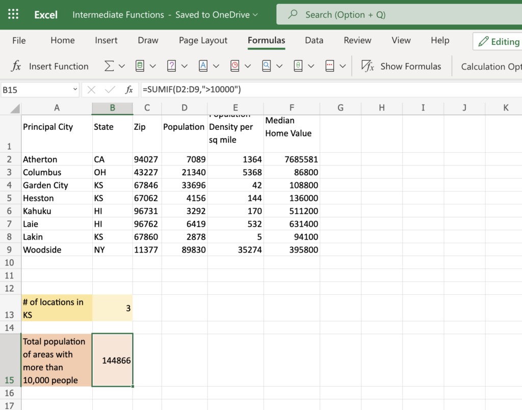
COUNTIF() and SUMIF() Worksheet
It’s often very useful to count or total only items or rows that meet certain criteria. The COUNTIF() and SUMIF() functions are perfect for this.
They work just like their non-if versions except you can give them a logical test. Just enter the range as usual then a comma and then the logical test.
Let’s start with COUNTIF(). We’ll find the number of locations in Kansas. This time we’ll use the
Enter your formula in B13
Enter the range: =COUNTIF(B2:B9
Now finish with the logical test. It needs to be in quotes. =COUNTIF(B2:B9,”=KS”)
You can also do it with your mouse with less typing if you prefer. Watch the video to see how.
Now find the total population of areas with more the 10,000 people.
Use the SUMIF() function in B15
Is very much like the COUNTIF() example except the range will be D2:D9 and Population>10000.
The worksheet should look like this when you finish.
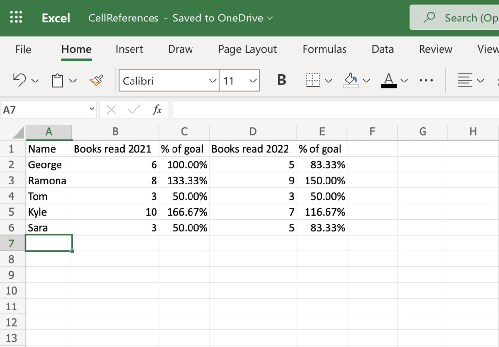
Many times it is needed to use values from other cells to calculate totals, averages, or other useful information. This is a basic feature of all spreadsheets. In this lesson you will learn how to work with reference that change as formulas are copied to new cells, references that don’t change when they are copied to other cells, and even cell that are on a different worksheet.
From the main office.com screen, upload the file from your download folder.
Relative Cell References
Relative references change when a formula is copied to another cell.
By default, all cell references are relative references. When copied across multiple cells, they change based on the relative position of rows and columns.
Copy the formula to find the total books read from cell D2 (=B2+C2) down to the cells under it. The cell reference will change to match the amount of movement. If you paste the formula three cell down, the formula will refer to cells three cells down from the ones that were originally referred to. This works in any direction, up, down, left, or right.
Relative references are especially convenient whenever you need to repeat the same calculation across multiple rows or columns.
Relative References
Absolute Cell References
Absolute references remain constant no matter where they are pasted.
There may be times when you do not want a cell reference to change when pasting a formula to other cells. Unlike relative references, absolute references do not change when copied or pasted. You can use an absolute reference to keep a row and/or column constant.
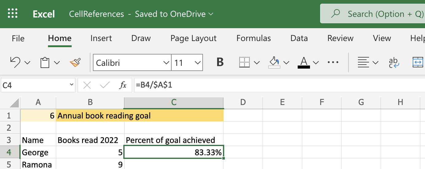
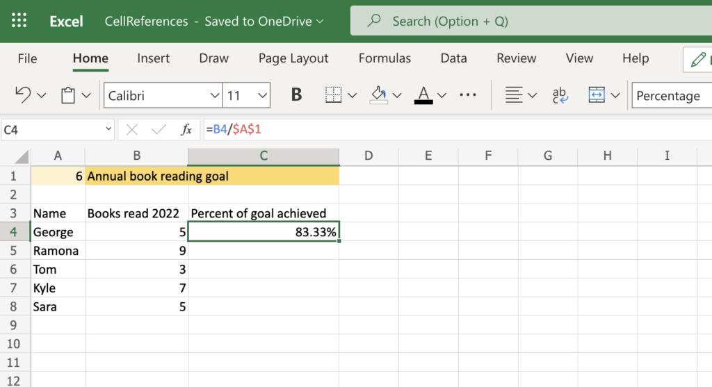
Absolute References
In this worksheet, the formula in cell C4 is =B4/$A$1. Cell A1 contains the book reading goal (6). If we copy this formula down to the next row below, Excel will change the formula to =B5/$A$1. Notice that the reference to A1 using the dollar signs stayed the same. A1 will ALWAYS contain the book reading goal so we want it to always stay the same in the formula and not change. We want THAT value to remain ABSOLUTE. We tell Excel this by putting a $ in front of the “A” and the “1” in the first formula. Then we copy the formula down and only items without a $ in front will change.
Experiment with leaving the dollar signs out of the formula in C4 and then copy and paste it down. Then change it back to the correct way.
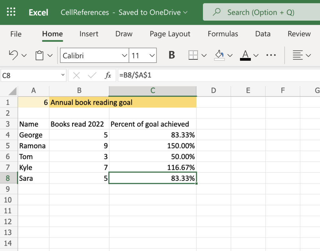
The following picture shows how it should look if done correctly.
Completed Absolute References Worksheet
Other Worksheet References
Excel allows you to refer to any cell on any worksheet, which can be especially helpful if you want to reference a specific value from one worksheet to another. To do this, you’ll simply need to begin the cell reference with the worksheet name followed by an exclamation point (!). For example, if you wanted to reference cell A1 on Sheet1, its cell reference would be Sheet1!A1.
If a worksheet name contains a space, you will need to include single quotation marks (‘ ‘) around the name. For example, if you wanted to reference cell A1 on a worksheet named Absolute References, its cell reference would be ‘Absolute References’!A1.
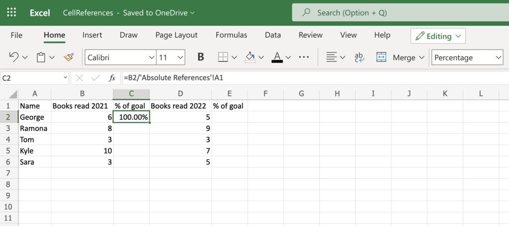
Look at the formula in C2 on the “Other Worksheet References” worksheet. It is referencing the book reading goal on the “Absolute References” worksheet.
Other Worksheet References
This formula works great! But if you copy it and paste it down on C3 through C6 it won’t work. Can you see why? Can you fix it?
The A1 part of the formula =B2/’Absolute References’!A1 is a relative reference and will need changed to be absolute. Try =B2/’Absolute References’!$A$1. Does that work?
When you have the formulas in column C working correctly, write a formula in E2 that will figure the percent of goal achieved for 2022. Then copy and paste it into the remaining cells in column E.
This is what it should look like when you are finished.
Competed Other Worksheet References
Feel free to change the book goal in cell A1 on the “Absolute References” worksheet and note how the % of goal numbers change on that worksheet as well as on the “Other Worksheet References” worksheet.
Great work! Now you know how to reference values in other cells!
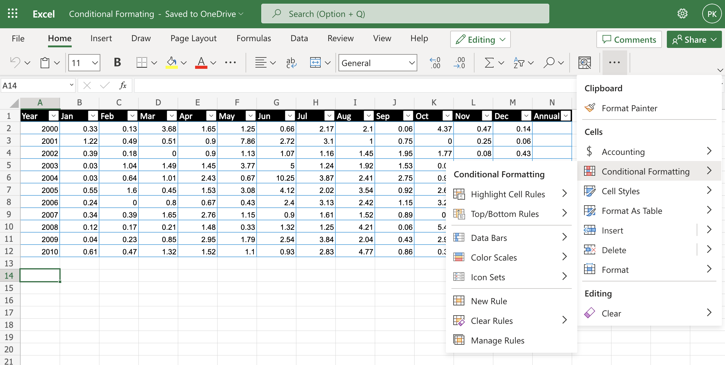
Conditional formatting is a wonderful way to draw attention to specific data. It also if very effective at highlighting differences in cell values. You will find other great uses for conditional formatting as you continue to use Excel.
From the main office.com screen, upload the file from your download folder.
Data Bars Worksheet
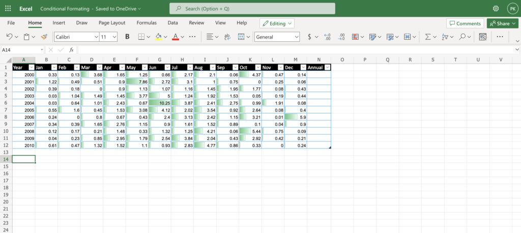
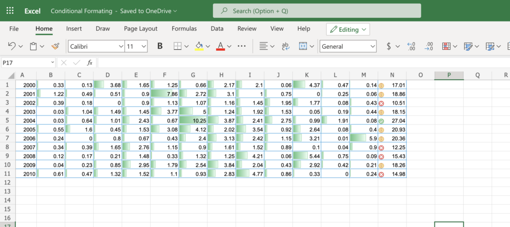
Add data bars to the month columns. This is a really easy way to draw attention to the difference in rainfall between months and years.
Select all 12 months in all 10 years.
On the “Home” menu, select Conditional Formatting -> Data Bars -> Green Data Bar in the Gradient Fill section.
The following video shows how to access the Conditional Formatting menu.
Conditional Formatting
Here is a screen shot of the what it should look like when you are done.
Data Bars
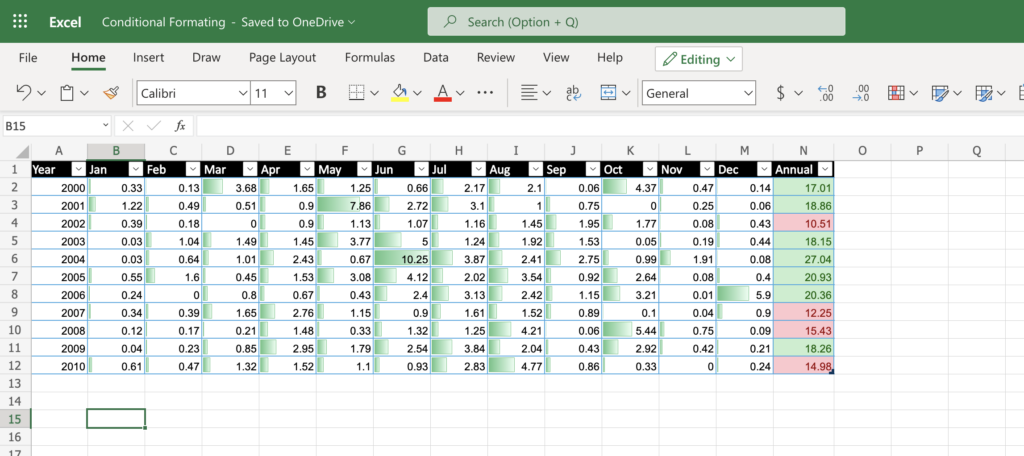
Highlight Cells Worksheet
Fill Column N (Annual) in the table using the SUM function.
Set Conditional Formatting for the values in Column N (Annual) to Highlight the cells to have a Red Fill if the annual rainfall is below 16″ and a Green Fill if the annual rainfall is equal to or above 16″.
Select Conditional Formatting -> Highlight Cell Rules -> Less Than.
Enter 16 in the last box of the rule.
In the “format with” drop down, select “light red fill with dark red text” if not all ready selected.
Click done.
Click the “plus” sign to add another rule.
Select greater than or equals to.
Enter 16 once again.
In the “format with” drop down, select “green fill with dark green text”
Click done.
Highlight Cells
Icon Sets Worksheet
First of all we will clear the formatting from column N (Annual) and replace it with an icon set. Icon sets automatically change based on how an individual cell compares to all the rest. This is a very easy way to emphasize cells that have high or low values.
With the same cells still selected, Select Conditional Formatting -> Icons Sets.
Choose one three symbols (Circled) from the Indicators section.
Still with the same cells selected, Select Conditional Formatting -> Manage Rules.
Click the little pencil icon to edit the rule.
Experiment with a few different icon sets. Stop when you feel you have found the icon set that best highlights low, average, and high rain fall years. There is not a right or wrong icon set. It is a matter of what you feel best highlights the information to your audience.
Icon Sets
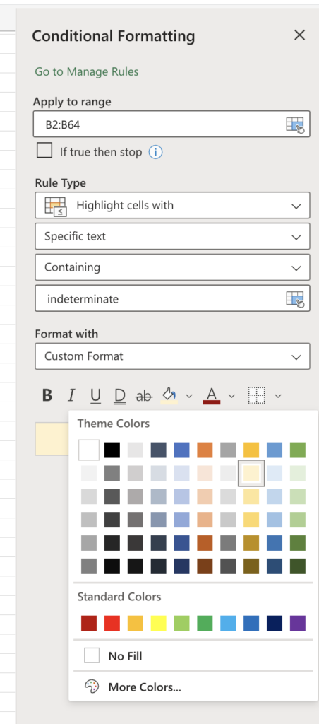
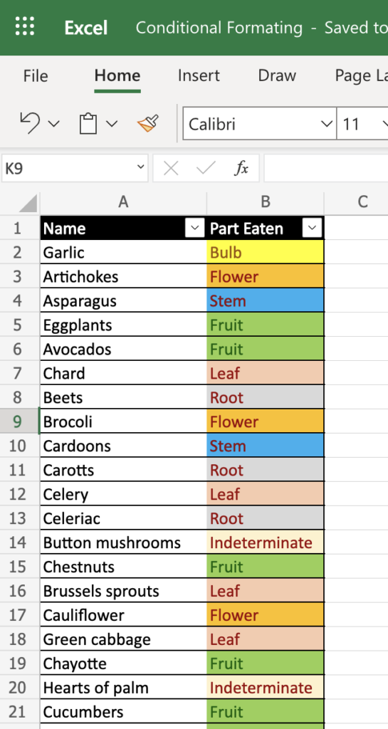
Highlight Text Worksheet
This list shows what part of common fruits and vegetables is eaten. Using what you have learned in the previous exercises, highlight each eatable part with a different background color.
You will need to start by selecting Conditional Formatting -> Highlight Cell Rules -> Text that contains.
Experiment with the highlighting options. You may find it best to use a custom fill color. You will find this on the menu of icons below the “format with” drop down.
Add rules as needed.
Highlight Text
Above Average worksheet
In this exercise you will find the average number of chapters in the books of the New Testament. Then you will highlight the book the have more chapters than average.
Use a Bible to finish filling in the books of the New Testament along with how many chapters each one has.
Use the AVERAGE function to show the average number of chapters at the bottom of the “# of chapters” column.
Use the “Conditional Formatting -> Top/Bottom Rules -> Above average” conditional formatting rule to highlight the books that have above average chapters. You can choose which formatting style you think is most appropriate.